5 Probability Theory

5.1 Conditional Probability and Independence

Suppose we have a probability model associated to a sample space \(S\). If we are told some event \(B\) has occurred, how would the probability of other events change? Calculating a new probability for event \(A,\) given that \(B\) has occurred is called a conditional probability, and will be denoted \(P(A|B)\).

For instance, Let \(X\) denote the outcome if we roll a fair six-sided die. Let \(A\) be the event that we roll a 4, and \(B\) the event that we roll an even number. Since the die is fair, we expect that \(P(A) = 1/6\). Now suppose that the die is rolled and we are told that the event \(B\) has occurred. This leaves only three possible outcomes: 2, 4, and 6. The new, conditional probability of \(A\) given \(B\) would be \(P(A|B) = 1/3.\)

Definition 5.1 The conditional probability of an event \(A,\) given that an event \(B\) has occurred, denoted \(P(A|B),\) is \[\begin{equation} P(A|B) = \frac{P(A \cap B)}{P(B)}, \tag{5.1} \end{equation}\] provided that \(P(B) > 0\).

Example 5.1 For the 2023 Major League Baseball season, 328 hitters had at least 250 plate appearances. In this group, 71% of them hit at least 10 HR for the season, and 31% of them hit at least 20 HR. If you pick a player from this group at random, and you are told they hit over at least 10 HR, what is the probability that they hit at least 20 HR?

Let \(A\) be the event that the player hits at least 20 HR, and \(B\) the event that a player hit at least 10. Then we have been asked to find \(P(A|B)\). Note that \(A\) is a subset of \(B\) (if a player hit at least 20, then they also hit at least 10), so \(A \cap B\) = \(A,\) and it follows that \[\begin{align*} P(A|B) &= \frac{P(A \cap B)}{P(B)} \\ &= \frac{P(A)}{P(B)} \\ &= \frac{.31}{.71}\\ &\approx .437. \end{align*}\]

Note that from the conditional probability formula,

\[P(A \cap B) = P(B) \cdot P(A~|~B), \text{ provided }P(B)>0,\] and that

\[P(A \cap B) = P(A) \cdot P(B~|~A), \text{ provided }P(A)>0.\]

Definition 5.2 Two events are called independent if any of the following statements holds:

\[\begin{align*} P(A~|~B) &= P(A) \\ P(B~|~A) &= P(B) \\ P(A \cap B) &= P(A)\cdot P(B) \end{align*}\]

Example 5.2 The chance experiment “roll a 6-sided die” has sample space \(S = \{1, 2, 3, 4, 5, 6\}\). Consider the events

\[\begin{align*} A &= \{1,3,5\}\\ B &= \{1\}\\ C &= \{2\}\\ D &= \{1,2\} \end{align*}\]

Then \(P(A) = 1/2, P(B) = 1/6, P(C) = 1/6,\) and \(P(D) = 1/3.\)

Claim 1: \(A\) and \(D\) are independent events.

Reason 1: Well, \(A \cap D = \{1\},\) so \[P(A~|~D) = \frac{P(A\cap D)}{P(D)} = \frac{1/6}{1/3} = 1/2 = P(A).\] Claim 2: \(B\) and \(C\) are not independent events.

Reason 2: \(B \cap C = \emptyset,\) so \[P(B~|~C) = \frac{P(B\cap C)}{P(C)} = \frac{0}{1/6} = 0 \neq P(B).\]

These simple examples help me remember that for events associated to a sample space,

independent is different than disjoint!

In this example \(A\) and \(D\) are independent but not disjoint, while \(B\) and \(C\) are disjoint but not independent.

Example 5.3 Suppose over the last five years, 10% of all people in a town who have hired a plumber to do some work have been unhappy with the job that was done. One of the plumbers in the town is Frances. Frances has done 40% of the plumbing jobs in town over these five years, and 25% of all plumbing jobs that left the customer unhappy have been done by Frances.

Find the probability that a customer will be unhappy with the results if they hire Frances?

We begin by translating what we know and what we want into symbols and probability notation.

Let \(S = \{ \text{all plumbing jobs in the town over the last 5 years} \}.\)

Let \(A = \{ \text{jobs handled by Frances} \}.\)

Let \(B = \{ \text{jobs in which the customer is unhappy} \}.\)

What do we want? \(P(B~|~A).\)

When do we want it? Now! So let’s write down what we know.

What do we know?

• 10% of the jobs have left the customer unhappy \(~~\Rightarrow~~~~ P(B) = 0.1\).
• Frances has done 40% of all jobs \(~~\Rightarrow~~~~ P(A) = 0.4\).
• 25% of all complaints dealt with Frances \(~~\Rightarrow~~~~ P(A~|~B) = 0.25\).

Well, \[\begin{align*} P(B~|~A) &= \frac{P(A\cap B)}{P(A)} \\ &= \frac{P(A ~|~B)\cdot P(B)}{P(A)} \\ &= \frac{(0.25)(0.1)}{(0.4)} \\ &= 0.0625. \end{align*}\]

Ok, there is about a 6 percent chance that a customer will be unhappy with their plumbing job if they hire Frances.

An irresponsible person who wants to be intentionally misleading could rant in all caps “25 PERCENT OF UNHAPPY CUSTOMERS HIRED FRANCES!!!” Let’s be better than that. Knowing the full context here, which includes what proportion of the town’s plumbing jobs have gone to Frances, is necessary to establish how effective Frances has been as a plumber these last five years.

Example 5.4

Roll 2 6-sided dice. What is the probability that both values are less than 3?

We assume the two dice are independent. (What appears on one die is independent of what appears on the other.)

Let \(A = \{ \text{first die is less than 3}\}\) and \(B = \{ \text{second die is less than 3}\}.\)

“Less than 3” means “1 or 2” so \(P(A) = P(B) = 2/6 = 1/3.\) The question asks for \(P(A \cap B).\) Since \(A\) and \(B\) are independent, \[P(A \cap B) = P(A)\cdot P(B) = (1/3)\cdot(1/3) = 1/9.\]

We remark that we can also use counting techniques to find this probability directly, as in Section 4.6, as follows.

The sample space \(S\) of this chance experiment consists of all possible rolls of the two dice. That is, \(S\) consists of all ordered pairs of the form \((i,j)\) with \(i, j \in \mathbb{N}\) and \(1\leq i, j \leq 6,\) and \(|S| = 6^2\). The event of interest, \(E,\) consists of all rolls \((i,j)\) in \(S\) such that \(i, j \leq 2\). So, \(|E| = 2^2,\) and \(P(E) = 4/36 = 1/9\).

So, thinking of the chance experiment as a sequence of independent events we calculate the probability of interest as \(\frac{2}{6} \cdot \frac{2}{6},\) and thinking of the probability via the “(outcomes of interest)/(all possible outcomes)” approach we think of the probability as \(\frac{2\cdot 2}{6 \cdot 6}\).

Example 5.5 Roll a regular 6-sided die until a 4 comes up. What is the probability that this occurs on the 8th roll?

The values of the rolls are independent events, the probability of not rolling a four on a given roll is 5/6, and the probability of rolling a 4 is 1/6. It follows that the probability of rolling 7 non-4s followed by one 4 is \[P(\text{first 4 on roll 8}) = \left(\frac{5}{6}\right)^7 \cdot \left(\frac{1}{6}\right).\] More generally, the probability that our first 4 comes up on roll \(n\) (for any \(n \in \mathbb{N}\)) will be \[P(\text{first 4 on roll }n) = \left(\frac{5}{6}\right)^{n-1} \cdot \left(\frac{1}{6}\right).\]

5.2 Two Laws of Probability

Theorem 5.1 Suppose \(A\) and \(B\) are two events.

1. Multiplicative Law of Probability: \[\begin{align*} P(A \cap B) &= P(A)\cdot P(B~|~A) \\ &= P(B) \cdot (A~|~B) \end{align*}\]

2. Additive Law of Probability: \[P(A\cup B) = P(A) + P(B) - P(A \cap B).\]

Proof.

1. This proof follows directly from the definition of conditional probability (5.1).

2. For finite sets \(A\) and \(B,\) we know \[|A \cup B| = |A| + |B| - |A \cap B|,\] from which the result follows.

More generally, for any sets \(A\) and \(B,\) the union \(A \cup B\) can be decomposed into disjoint sets: \(A \cup B = A \cup (\overline{A} \cap B).\) So, \[P(A \cup B) = P(A) + P(\overline{A} \cap B).\]

Similarly, we can decompose the set \(B\) into disjoint sets as follows: \(B = (\overline{A} \cap B) \cup (A \cap B).\) So \[P(B) = P(\overline{A}\cap B) + P(A \cap B).\] Combining these two probability equations we see \[P(A \cup B) = P(A) + \left[P(B)-P(A\cap B)\right],\] which completes the proof.

Next, consider three events, \(A_1, A_2, A_3\). Notice that

\[\begin{align*} P(A_1 \cap A_2 \cap A_3) &= P((A_1\cap A_2) \cap A_3) \\ &= P(A_1 \cap A_2) \cdot P(A_3~|~A_1 \cap A_2)\\ &= P(A_1) \cdot P(A_2~|~A_1) \cdot P(A_3~|~A_1 \cap A_2). \end{align*}\]

This formula may be extended to the intersection of any number of sets.

\[\begin{equation} P(A_1 \cap \cdots \cap A_k) = P(A_1) \cdot P(A_2 ~|~ A_1) \cap \cdots \cap P(A_k ~|~ (A_1 \cap \cdots \cap A_{k-1})) \tag{5.2} \end{equation}\]

Example 5.6 Flip over 4 cards from a regular 52-card deck. What is the probability they are all hearts?

We flip the cards over one at a time, and define the four events \(A_i\) = the event that card \(i\) is a hearts, for \(i = 1, 2, 3, 4\).

We want the probability that all four events occur. That is, we want \(P(A_1 \cap A_2 \cap A_3 \cap A_4),\) and we find this using Equation (5.2).

\[\begin{align*} P(A_1 \cap A_2 \cap A_3 \cap A_4) &= P(A_1) \cdot P(A_2 ~|~ A_1) \cdot P(A_3 ~|~ A_1 \cap A_2) \cdot P(A_4 ~|~ A_1 \cap A_2 \cap A_{3})\\ &= \frac{13}{52} \cdot \frac{12}{51} \cdot \frac{11}{50} \cdot \frac{10}{49} \\ &\approx 0.0026. \end{align*}\]

Example 5.7

Find the probability that a random 4 digit number has distinct odd digits.

Two notes: We have 5 odd digits, and the leading (thousands) digit of a 4-digit number cannot be 0.

Using the multiplicative law of probability we calculate the probability of a sequence of events and multiply them:

• The probability that the leading digit is odd: 5/9.
• The probability that the 2nd digit is odd, given the first was: 4/10.
• The probability that the 3rd digit is odd, given the first two were: 3/10.
• The probability that the 4th digit is odd, given the first three were: 2/10.

By the multiplicative law of probability, the probability that a random 4-digit number has distinct odd digits is \[\frac{5}{9} \cdot \frac{4}{10} \cdot \frac{3}{10} \cdot \frac{2}{10} \approx 0.0133.\]

We have three corollaries to Theorem 5.1.

Corollary 5.1 For any event \(A,\) \[P(\overline{A}) = 1 - P(A).\]

Proof. By the additive law, \[P(A \cup \overline{A}) = P(A) + P(\overline{A})-P(A \cap \overline{A}).\] Since \(A\cup \overline{A} = S\) and \(A \cap \overline{A} = \emptyset,\) \(P(A \cup \overline{A}) = 1\) and \(P(A \cap \overline{A}) = 0,\) so \[1 = P(A) + P(\overline{A}),\] and the result follows.

Corollary 5.2 If \(A\) and \(B\) are disjoint events, then \(P(A \cup B) = P(A) + P(B).\)

Proof. Since \(A\cap B = \emptyset,\) \(P(A \cap B) = 0\) and the result follows from the Additive Law of Probability.

Corollary 5.3 For three events \(A, B, C\).

The probability of their union is

\[\begin{align*} P(A \cup B \cup C) &= P(A)+P(B)+P(C)\\ &~~~~ - [P(A\cap B) + P(A \cap C) + P(B \cap C)]\\ &~~~~ + P(A \cap B \cap C). \end{align*}\]

The probability of their intersection is \[P(A \cap B \cap C) = P(A) \cdot P(B~|~A) \cdot P(C ~|~ A \cap B).\]

Proof. First we tackle the union case by appealing to the additive law of probability twice, along a the distributive law of sets.

\[\begin{align*} P(A \cup B \cup C) &= P(A \cup (B \cup C)) \\ &= P(A) + P(B \cup C) - P(A \cap (B \cup C)) \\ &= P(A) + [P(B) + P(C)- P(B \cap C)] - P((A\cap B) \cup (A \cap C)) \\ &= P(A) + P(B) + P(C) - P(B \cap C) \\ &~~~~ - [P(A \cap B)+ P(A \cap C)-P((A \cap B) \cap (A \cap C))]\\ &= P(A) + P(B) + P(C) \\ &~~~~ - [P(A\cap B) + P(A \cap C) + P(B \cap C)] \\ &~~~~ + P((A \cap B) \cap (A \cap C)) \end{align*}\]

from which the result follows since \(A \cap B \cap A \cap C = A \cap B \cap C\).

For the intersection case, by definition of conditional probability the right hand side of the equation is \[\text{RHS } = P(A) \cdot \frac{P(A \cap B)}{P(A)} \cdot \frac{P(C\cap A\cap B)}{P(A \cap B)},\] and the result follows by cancellation.

5.3 Event-Composition Method

In some examples in this chapter we’ve been using a method for calculating probabilities called the event-composition method, which can be described as follows.

Event-Composition Method: Describe the sample space and relevant events; write down what information we’re given regarding probabilities etc. via the symbols representing these events; Express what we want to know via these symbols, and use our probability laws to use what we know to determine what we want.

Example 5.8 Two regular 6-sided dice are rolled until we roll a sum of 4 or a sum of 7.

What is the probability that we roll a 4 before we roll a 7?

We define two key events:

• \(A\): we roll a sum of 4; and
• \(B\): we do not roll a 4 or 7.

From our handy \(6 \times 6\) grid describing all possible sums when rolling 2 dice (Example 3.3), we know \[P(A) = \frac{3}{36}, ~~P(B) = \frac{27}{36}.\]

In this game we roll the dice until we roll a 4 or a 7, and we win if we roll a 4 before rolling a 7.

There is no limit to how many rolls we might need in order to win. We might win on the 1st roll, or the 2nd roll, or the 3rd roll, or the 4th roll, … etc. In fact, for each \(n \in \mathbb{N},\) we might win on roll \(n\).

Put another way, we can partition the event of winning into a countably infinite collection of mutually disjoint events: winning on roll 1, winning on roll 2, winning on roll 3, etc. Then, \[P(\text{winning}) = \sum_{n=1}^\infty P(\text{winning on roll }n).\]

The probability of winning on the 1st roll is \(P(A)\).

The probability of winning on the 2nd roll is \(P(B) \cdot P(A)\) (no 4 or 7 on 1st roll and yes 4 on the 2nd roll).

The probability of winning on the 3rd roll is \(P(B) \cdot P(B) \cdot P(A),\) and, more generally, the probability of winning on roll \(n\) is \[P(B)^{n-1}\cdot P(A).\]

The sum of these probabilities is an honest-to-goodness-living-in-the-wild geometric series:

\[\begin{align*} P(\text{4 before 7}) &= \sum_{n=1}^\infty P(B)^{n-1}P(A)\\ &= P(A)\sum_{n=0}^\infty P(B)^n\\ &= \frac{3}{36}\sum_{n=0}^\infty \left(\frac{27}{36}\right)^n \end{align*}\]

As a reminder, the sum of a geometric series is given by \[\begin{equation} \sum_{n=0}^\infty r^n = \frac{1}{1-r} \text{ if } |r| < 1 \tag{5.3} \end{equation}\]

Using this formula with \(r = 27/36,\) we see the probability that we roll a 4 before a 7 is \[P(\text{4 before 7}) = \frac{3}{36}\cdot \frac{1}{1-(27/36)} = \frac{1}{3}.\]

5.4 Bayes’ Rule

Definition 5.3 A collection \(\{B_1, B_2, \ldots, B_n\}\) of nonempty subsets of \(S\) is called a partition of \(S\) provided that

1. \(S = B_1 \cup B_2 \cup \cdots \cup B_n,\) and
2. the collection is pairwise disjoint.

Theorem 5.2 (Law of Total Probability) Assume \(\{B_1, B_2, \ldots, B_k\}\) is a partition of the sample space \(S,\) and \(P(B_i) > 0\) for each \(i = 1, 2, \ldots k\). Then for any event \(A,\) \[P(A) = \sum_{i=1}^k P(A~|~B_i)\cdot P(B_i).\]

Proof. Notice that as a set, \[\begin{align*} A &= A \cap S \\ &= A \cap (B_1 \cup B_2 \cup \cdots \cup B_k) \\ &= (A \cap B_1) \cup (A \cap B_2) \cup \cdots \cup (A \cap B_k). \end{align*}\]

Furthermore, since the \(B_i\) are pairwise disjoint, the \((A \cap B_i)\) are pairwise dijoint as well, and by the additive law of probability \[P(A) = \sum_{i = 1}^k P(A \cap B_i).\]

The result then follows since each \(P(A \cap B_i) = P(A~|~B_i)\cdot P(B_i)\).

Example 5.9 An ad agency notices

• 1 in 50 potential buyers of a particular product sees an advertisement for it on television
• 1 in 5 potential buyers sees the ad on YouTube.
• 1 in 100 sees the ad on both TV and YouTube.
• 1 in 3 potential buyers actually purchase the product after seeing an ad, and
• 1 in 10 potential buyers buy it without seeing an ad.

What is the probability that a radnomly selected potential buyer will purchase the product?

We define relevant events for the sample space \(S = \{ \text{ all potential buyers }\}\). In particular, we let

• \(A\) = the set of potential buyers who purchase the product,
• \(B\) = the set of potential buyers who see the ad on TV,
• \(C\) = the set of potential buyers who see the ad on YouTube.

Next we translate what we know and what we want into symbols.

What we want: \(P(A)\).

What we know:

• \(P(B) = 1/50,\)
• \(P(C) = 1/5,\)
• \(P(B \cap C) = 1/100,\)
• \(P(A ~|~ B \cup C) = 1/3,\) and
• \(P(A ~|~ \overline{B \cup C}) = 1/10.\)

We also know by the additive law of probability that

\[P(B \cup C) = \frac{1}{50} + \frac{1}{5} - \frac{1}{100} = \frac{21}{100},\] so by Corollary 5.1, \[P(\overline{B \cup C}) = 1 - \frac{21}{100} = \frac{79}{100}.\] Finally, notice that since \(B \cup C\) and \(\overline{B \cup C}\) partition the sample space, \[A = \left[A \cap (B \cup C)\right] \cup \left[A \cap (\overline{B \cup C})\right],\] where these two sets are disjoint.

By the Law of Total Probability,

\[\begin{align*} P(A) &= P(A \cap (B \cup C)) + P(A \cap (\overline{B \cup C)})\\ &= P(B \cup C) \cdot P(A ~|~ B \cup C) + P(\overline{B \cup C})\cdot P(A~|~\overline{B \cup C})\\ &= \frac{21}{100} \cdot {1}{3} + \frac{79}{100}\cdot {1}{10} \\ &= \frac{7}{100} \cdot \frac{7.9}{100} \\ &= 0.149. \end{align*}\]

Example 5.10 Suppose you have taken a test for a deadly disease. The doctor tells you that the test is quite accurate in that if you have the disease then the test will correctly tell you that you have the disease 100% of the time. However, if you don’t have the disease, the test will very occasionally (1 time in 10) mistakenly tell you that you have it.

The test comes back positive (it says you have the disease)! Are you worried!? In particular, can you estimate the probability that you actually have the disease given that the test came back positive?

What information were we given? What information do we want?

We were given:

• The probability of a positive test given I have the disease is 1.
• The probability of a positive test given I do not have the disease is 0.1

We want:

• The probability I have the disease given that I have a positive test.

Let \(A\) denote the event that I have a positive test, \(B\) the event that I have the disease.

Then I want \(P(B|A)\) and I know \(P(A|B) = 1\) and \(P(A|\overline{B}) = 0.1.\)

It turns out I need more information than I’ve been given to answer this question, as the following scenarios demonstrate.

Scenario 1: Suppose the population consists of 100 people, and 50 people, in fact, have the disease (blue - healthy, red - sick in the figure below). Then, if we tested each individual we would find 55 positive tests (the circled dots below) (all 50 of the sick people would test positive, and 10% of the 50 healthy people, so 5 healthy people would also test positive.)

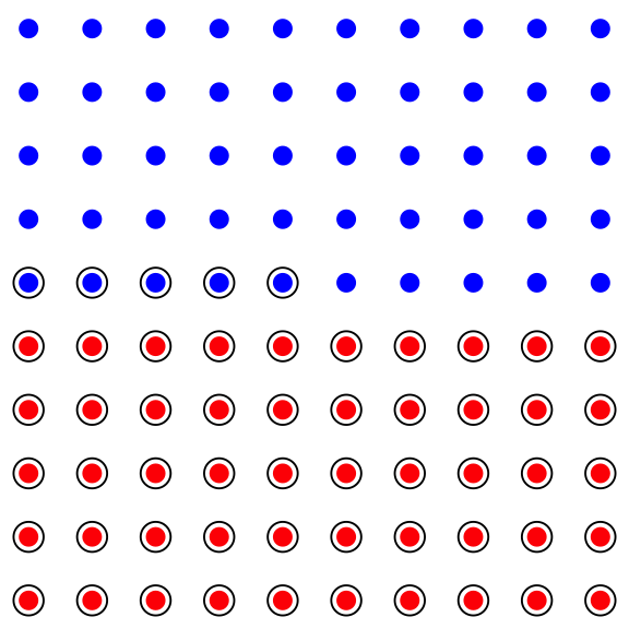
Figure 5.1: 50% of population has the disease

In this scenario, given that I tested positive, there is a 50/55 chance that I have the disease.

Scenario 2: Suppose the population consists of 100 people, and 1 person, in fact, has the disease (blue - healthy, red - sick in the figure below). Then, if we tested each individual we would find about 11 positive tests (the circled dots below) (the one sick people would test positive, and 10% of the 99 healthy people, so about 10 healthy people would also test positive.)

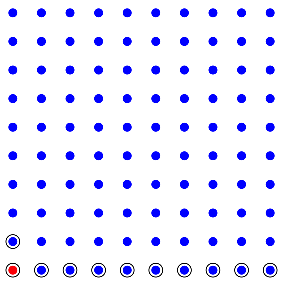
Figure 5.2: 1% of population has the disease

In this scenario, given that I tested positive, there is a 1/11 chance that I have the disease.

So, it seems to answer the question in this example, it is important to know what percentage of the population have the disease. Baye’s Theorem below tells us that this is all the additional information we need.

Theorem 5.3 (Bayes' Rule) Assume \(\{B_1, B_2, \ldots, B_k\}\) is a partition of the sample space \(S,\) and \(P(B_i) > 0\) for each \(i = 1, 2, \ldots k\). Then for any particular \(B_j,\) \[P(B_j ~|~ A) = \frac{P(A~|~B_j)\cdot P(B_j)}{\sum_{i=1}^k P(A~|~B_i)\cdot P(B_i)}.\]

Example 5.11 A grocery store has an apple bin. 70% of the apples are Liberty, and 30% are Braeburn. From past experience, we know that 8% of Liberty apples are bad, and 15% of Braeburn apples are bad. Suppose you pick an apple at random and find it is bad. What is the probability that the apple is a Braeburn?

We define our relevant sets.

• \(S\) = all apples in the bin
• \(B_1\) = all Liberty apples in \(S\)
• \(B_2\) = all Braeburn apples in \(S\) (and the \(B_i\) partition \(S\)!)
• \(A\) = bad apples in \(S\).

We know:

• \(P(B_1) = .7,\) and \(P(B_2) = .3\)
• \(P(A~|~B_1) = .08,\) and \(P(A~|~B_2) = .15\).

We want:

• \(P(B_2 ~|~ A)\).

This task calls for Bayes’ Rule.

\[P(B_2~|~A) = \frac{P(A~|~B_2)\cdot P(B_2)}{P(A~|~B_1)\cdot P(B_1)+P(A~|~B_2)\cdot P(B_2)}.\] We know each probability in the right-hand side of the equation: \[P(B_2~|~A) = \frac{(.15)(.3)}{(.08)(.7)+(.15)(.3)} \approx .446.\] About a 44% chance that if we drew a bad apple it’s a Braeburn.

We can also use a tree diagram to arrive at this answer:

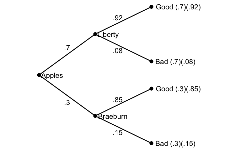
Figure 5.3: Picking an Apple

From the diagram, the probability of picking a bad apple is \((.7)(.08) + (.3)(.15)\) and the probability of picking a bad Braeburn is \((.3)(.15),\) so the probability of having picked a Braeburn, given we picked a bad apple is \[\frac{(.3)(.15)}{(.7)(.08) + (.3)(.15)}.\]

Example 5.12 Two methods, \(A\) and \(B\) are available for teaching a certain skill at a factory. The failure rate for \(A\) is 20%, and for \(B\) is 10%. However, \(B\) is more expensive and is used only 30% of the time (\(A\) is used the other 70%). A worker was taught the skill by one of the methods but failed to learn it correctly. What is the probability they were taught by Method \(A\)?

Let \(S\) denote the sample space of all workers who have been trained in this skill.

We have this partition of \(S\):

• \(A\) = those taught by method \(A\)
• \(B\) = those taught by method \(B\).

We also have \(F\) = those who fail to learn the skill correctly.

We want: \(P(A~|~F)\).

We know: \(P(A) = .7,\) \(P(B) = .3,\) \(P(F~|~A) = .2,\) and \(P(F~|~B) = .1\).

Using Bayes’ Rule, \[\begin{align*} P(A~|~F) &= \frac{P(A)\cdot P(F~|~A)}{P(A)\cdot P(F~|~A)+P(B)\cdot P(F~|~B)}\\ &= \frac{(.7)(.2)}{(.7)(.2)+(.3)(.1)}\\ &\approx .82. \end{align*}\] Given a worker failed to learn the skill, there is about an 82% chance they had been taught by Method \(A\).

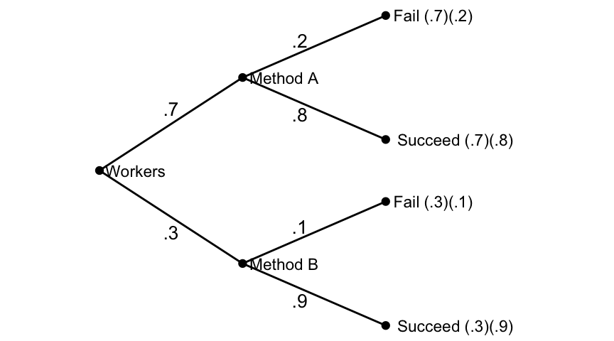
Figure 5.4: Learning by a Method