11 Moment Generating Functions
Recall by Definition 8.2, the moment-generating function (mgf) associated with a discrete random variable \(X,\) should it exist, is given by \[m_X(t) = E(e^{tX})\] where the function is defined on some open interval of \(t\) values containing 0. The same definition applies to continuous random variables. We have seen that this mgf encodes information about \(X\): the \(k\)th derivative of \(m\) evaluated at \(t = 0\) gives us the \(k\)th moment. That is, for \(k = 1,2,3,\ldots,\) \[m_X^{(k)}(0) = E(X^k).\] In fact, it turns out that the mgf gives us all the information about a random variable \(X,\) per the following theorem, whose proof is beyond the scope of this course.
Theorem 11.1 Let \(m_X(t)\) and \(m_Y(t)\) denote the mgfs of random variables \(X\) and \(Y,\) respectively. If both mgfs exist and \(m_X(t) = m_Y(t)\) for all values of \(t\) then \(X\) and \(Y\) have the same probability distribution.
Example 11.1
Find the mgf for the standard normal random variable \(Z \sim N(0,1)\).
\[\begin{align*} m_Z(t) &= E(e^{tZ})\\ &= \int_{-\infty}^\infty \frac{1}{\sqrt{2\pi}}e^{-z^2/2}\cdot e^{tz}~dz\\ &= \frac{1}{\sqrt{2\pi}} \int_{-\infty}^\infty e^{tz-z^2/2}~dz\\ &= \frac{1}{\sqrt{2\pi}} \int_{-\infty}^\infty e^{-\frac{1}{2}(z-t)^2+\frac{1}{2}t^2}~dz &\text{complete the square}\\ &= e^{\frac{1}{2}t^2}\left[\frac{1}{\sqrt{2\pi}} \int_{-\infty}^\infty e^{-\frac{1}{2}(z-t)^2}~dz\right] \end{align*}\]
The bracketed portion of this last expression equals 1, for all \(t,\) since it is the integral of the density function of a \(N(t,1)\) distribution, so \[m_Z(t) = e^{\frac{1}{2}t^2},\] for all \(-\infty < t < \infty\).
More generally, for \(X \sim N(\mu,\sigma),\) one can show its mgf is
\[\begin{equation} m(t) = e^{\left(\mu t + \frac{\sigma^2}{2}t^2\right)} \tag{11.1} \end{equation}\]
We now return to the proof of Theorem 10.4, which we restate as the following lemma.
Lemma 11.1 If \(X\) is \(N(\mu,\sigma)\) and \(Z = \frac{X-\mu}{\sigma},\) then \(Z\) is \(N(0,1)\).
Proof. Let \(X\) be \(N(\mu,\sigma),\) and \(Z = \frac{X-\mu}{\sigma}\). Then the mgf for \(Z\) is
\[\begin{align*} m_Z(t) &= E\left[e^{tZ}\right]\\ &= E\left[e^{t\left(\frac{X-\mu}{\sigma}\right)}\right]\\ &= E\left[e^{\frac{Xt}{\sigma} - \frac{\mu t}{\sigma}}\right]\\ &= E\left[e^{Xt/\sigma} \cdot e^{-\mu t/\sigma}\right] \\ &= e^{-\mu t/\sigma}\cdot E\left[e^{Xt/\sigma}\right]\\ &= e^{-\mu t/\sigma}\cdot m_X(t/\sigma) \end{align*}\] This last step follows because \(\displaystyle E\left[e^{Xt/\sigma}\right]\) is the mgf of \(X\) evaluated at \(t/\sigma\). Then,
\[\begin{align*} m_Z(t) &= e^{-\mu t/\sigma}\cdot e^{\left(\mu (t/\sigma) + \frac{\sigma^2}{2}(t/\sigma)^2\right)} \\ &= e^{t^2/2} \end{align*}\]
But hey! This mgf is the mgf for \(N(0,1),\) so by Theorem 11.1, since \(Z = (X-\mu)/\sigma\) and \(N(0,1)\) have the same mgf, they have the same probability distribution.
Lemma 11.2 If \(Z\) is \(N(0,1)\) then \(Z^2\) is \(\chi^2(1)\).
The proof of this lemma is left for now.
Theorem 11.2 Let \(X_1, X_2, \ldots, X_n\) be independent random variables with mgfs \(m_1(t), m_2(t), \ldots m_n(t),\) respectively. If \(U = X_1 + X_2 + \cdots + X_n\) then \[m_U(t) = m_1(t) \cdot m_2(t) \cdot ~\cdots~ \cdot m_n(t).\]
Sketch of Proof:
\[\begin{align*} m_U(t) &= E\left[e^{tU}\right]\\ &= E\left[e^{t(X_1 + X_2 + \cdots X_n)}\right]\\ &= E\left[e^{tX_1}\cdot\ e^{tX_2} \cdot ~\cdots~ \cdot e^{tX_n}\right]\\ &= E\left[e^{tX_1}\right] \cdot E\left[e^{tX_2}\right] \cdot ~\cdots~ \cdot E\left[e^{tX_n}\right]\\ &= m_1(t) \cdot m_2(t) \cdot ~\cdots~ \cdot m_n(t) \end{align*}\]
That the \(E[~]\) distributes through the product in line 4 above follows since the \(X_i\) are assumed to be independent. The proof of this fact would be given in MATH 440.
Theorem 11.3 Let \(X_1, X_2, \ldots, X_n\) be independent normal random variables with \(X_i \sim N(\mu_i, \sigma_i),\) and let \(a_1, a_2, \ldots, a_n\) be constants. If \[U = \sum_{i=1}^n a_i X_i,\] then \(U\) is normally distribution with \[\mu = \sum_{i=1}^n a_i \mu_i ~~~ \text{ and } ~~~ \sigma^2 = \sum_{i=1}^n a_i^2 \sigma_i^2.\]
Proof. Since \(X_i\) is \(N(\mu_i,\sigma_i),\) \(X_i\) has mgf \[m_{X_i}(t) = e^{\left(\mu_it + \sigma_i^2t^2/2\right)}.\] For constant \(a_i,\) the random variable \(a_iX_i\) has mgf \[m_{a_iX_i}(t) =E(e^{a_iX_it}) = m_{X_i}(a_it) = e^{\left(\mu_ia_it + a_i^2\sigma_i^2t^2/2\right)}.\] Then by Theorem 11.2 and properties of exponents, for \(U = \sum a_i X_i,\) \[\begin{align*} m_U(t) &= \prod_{i=1}^n m_{a_iX_i}(t) \\ &= \prod_{i=1}^n e^{\left(\mu_ia_it + a_i^2\sigma_i^2t^2/2\right)}\\ &= e^{\left(t\sum a_i\mu_i + \frac{t^2}{2}\sum a_i^2\mu_i^2\right)} \end{align*}\]
But hey! This is the mgf for a normal distribution with mean \(\sum a_i \mu\) and variance \(\sum a_i^2 \sigma_i^2,\) so we have proved the result.
Theorem 11.4 Let \(X_1, X_2, \ldots, X_n\) be independent normal random variables with \(X_i \sim N(\mu_i, \sigma_i),\) and \(\displaystyle Z_i = \frac{X_i - \mu_i}{\sigma_i}\) for \(i = 1, \ldots, n\). Then \[U = \sum_{i=1}^n Z_i^2\] is \(\chi^2(n)\).
Example 11.2 Suppose the number of customers arriving at a particular checkout counter in an hour follows a Poisson distribution. Let \(X_1\) record the time until the first arrival, \(X_2,\) the time between the 1st and 2nd arrival, and so on, up to \(X_n,\) the time between the \((n-1)\)st and \(n\)th arrival. Then it turns out the \(X_i\) are independent, and each is an exponential random variable with density \[f_{X_i}(x_i) = \frac{1}{\theta}e^{-x_i/\theta},\] for \(x_i > 0\) (and 0 else). Find the density function for the waiting time \(U\) until the \(n\)th customer arrives.
Well \(U = X_1 + X_2 + \cdots + X_n,\) so by Theorem 11.2, \[m_U(t) = m_1(t)\cdot ~\cdots~ \cdot m_n(t) = (1-\theta t)^{-n}.\] But, hey! This is the mgf for a gamma\((\alpha = n, \beta = \theta)\) random variable so by Theorem 11.1, \(U\) is gamma\((n,\theta)\). So \[f_U(u) = \frac{1}{(n-1)!\theta^n}u^{n-1}e^{-u/\theta},\] for \(u > 0\) (and 0 else).
Example 11.3 If \(Y_1\) is \(N(10,.5)\) and \(Y_2\) is \(N(4,.2)\) and \(U = 100 + 7Y_1 + 3Y_2,\) how is \(U\) distributed, and what value marks the 90th percentile for \(U\)?
Theorem 11.3 says that \(U\) is normal with \[E(U) = 100 + 7 \cdot 10 + 3 \cdot 4 = 182,\] and \[V(U) = 0 + 7^2\cdot (.5)^2 + 3^2\cdot(.2)^2 = 12.61,\] so \(\sigma_U = \sqrt{12.61} = 3.55.\)
The 90th percentile can be found in R with the qnorm() function:
## [1] 186.5495Example 11.4
Find the moment-generating function for \(X ~\sim U(\theta_1, \theta_2)\).
\[\begin{align*} m_X(t) &= E(e^{tX})\\ &= \int_{\theta_1}^{\theta_2} e^{tx}\frac{1}{\theta_2-\theta_1}~dx\\ &= \frac{1}{\theta_2-\theta_1} \frac{1}{t}e^{tx}~\biggr|_{\theta_1}^{\theta_2} \\ &= \frac{e^{t(\theta_2-\theta_1)}}{t(\theta_2-\theta_1)}. \end{align*}\]
Example 11.5
Find the moment-generating function for \(X \sim \text{gamma}(\alpha,\beta)\) and compute \(E(X)\) and \(V(X)\).
\[\begin{align*} m_X(t) &= E(e^{tX})\\ &= \int_{0}^{\infty} e^{tx} \cdot \frac{1}{\beta^\alpha \Gamma(\alpha)}x^{\alpha-1}e^{-(x/\beta)}~dx\\ &= \frac{1}{\beta^\alpha \Gamma(\alpha)} \int_{0}^{\infty} x^{\alpha - 1}e^{-x(1/\beta-t)}~dx\\ &= \frac{1}{\beta^\alpha \Gamma(\alpha)} \cdot \left(\frac{1}{1/\beta - t}\right)^\alpha \Gamma(\alpha) \int_{0}^{\infty} \frac{x^{\alpha - 1}e^{-x(1/\beta-t)}}{\left(\frac{1}{1/\beta - t}\right)^\alpha \Gamma(\alpha)}\cdot ~dx\\ &= \frac{1}{\beta^\alpha \Gamma(\alpha)} \cdot \left(\frac{1}{1/\beta - t}\right)^\alpha \Gamma(\alpha) \end{align*}\]
The last integral above evaluates to 1 because it is the pdf for a \(\text{gamma}(\alpha,\beta)\) distribution! After simplifying we obtain \[m_X(t) = (1-\beta t)^{-\alpha}.\]
With the mgf for a gamma random variable in hand, we can now derive its mean and variance, thus proving Theorem 10.5.
\[\begin{align*} m_X^\prime(t) &= -\alpha(1-\beta t)^{-\alpha-1}\cdot(-\beta) \\ &= \alpha\beta(1-\beta t)^{-\alpha-1}, \end{align*}\] so \[E(X) = m_X^\prime(0) = \alpha\beta.\] Turning to the second derivative, \[\begin{align*} m_X^{\prime\prime}(t) &= (-\alpha-1)\alpha\beta(1-\beta t)^{-\alpha-2}\cdot(\beta)\\ &= \alpha(\alpha+1)\beta^2(1-\beta t)^{-\alpha-2}, \end{align*}\] so \[E(X^2) = m_X^{\prime\prime}(0) = \alpha(\alpha+1)\beta^2.\] Thus, \[V(X) = E(X^2)-E(X)^2 = \alpha(\alpha+1)\beta^2 - (\alpha\beta)^2 = \alpha\beta^2.\]
Example 11.6 The average velocity of nails shot from a nail gun is 2000 ft/s. Suppose the velocity varies according to a gamma(4,500) distribution, so the probability density function is \[f(v) = \frac{v^3e^{-v/500}}{6 \cdot 500^4},\] for \(v > 0\).
We note that this nail gun has the following (alarming?) velocity distribution:
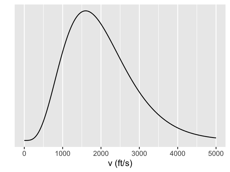
Figure 11.1: Nail gun velocity distribution
The kinetic energy \(K\) associated with a nail having mass \(m\) moving at velocity \(V\) is \(K = \frac{1}{2}mV^2\). What is \(E(K)\)?
\[\begin{align*} E(K) &= E(\frac{1}{2}mV^2)\\ &= \frac{1}{2}m E(V^2) \\ &= \frac{1}{2}m (\sigma_V^2 + \mu_V^2) \end{align*}\] Since \(V\) is gamme(4,500), \(\mu_V = 4 \cdot 500 = 2000\) (as we were told) and \(\sigma_V = 4\cdot 500^2,\) so \[E(K) = 2500000m \text{ units}.\]