14 Confidence Intervals
In many of the examples in Chapter 13 we built confidence intervals, interval estimators that specify the method for using a sample to calculate two numbers that form the endpoints of an interval that likely (with some pre-assigned probability) contains the paramter of interest.
14.1 Pivotal Quantities
Here is the general scene for a confidence interval for a parameter \(\theta\). We use a sample to determine the lower and upper confidence limit estimators, \(\hat{\theta}_L\) and \(\hat{\theta}_U\). If \[P(\hat{\theta}_L \leq \theta \leq \hat{\theta_U}) = 1 - \alpha\] the probability \(1-\alpha\) is called the confidence level.
One method for finding confidence intervals is called the pivotal method, which leverages a pivotal quantity, which is a quantity with two features:
- It is a function of the data \(X_1, \ldots, X_n\) and the parameter of interest \(\theta,\) and
- its probability distribution does not depend on \(\theta\).
Example 14.1 If a population mean \(\mu\) is the parameter of interest, and we have sample \(X_1, \ldots, X_n,\) then a good pivotal quantity, assuming \(X_i\) is approximately \(N(\mu,\sigma),\) is \[T = \frac{\overline{X}-\mu}{S/\sqrt{n}}.\] It meets both requirements here: it is a function of the data and the parameter \(\mu,\) and it lives in a \(t(n-1)\) distribution, which is independent of \(\mu\).
Example 14.2 If a population proportion \(p\) is the parameter of interest, and we have sample proportion \(\hat{p}\) (from a sample of size \(n\)), then the pivotal quantity \[Z = \frac{\hat{p}-p}{\sqrt{\hat{p}(1-\hat{p})/n}}\] is approximately \(N(0,1),\) a distribution independent of \(p\).
Example 14.3 Consider \(X_1, \ldots, X_n\) drawn from the uniform distribution \(U(0,\theta)\) and \(Y = \text{max}(X_1, \ldots, X_n)\). We proved in Example 13.1 that \[F_Y(y) = \left(\frac{y}{\theta}\right)^n ~~~\text{ and }~~~ f_Y(y) = \frac{n}{\theta^n}y^{n-1},\] for \(0 \leq y \leq \theta\). Now, let \(U = \frac{1}{\theta}Y,\) which is just a function of the data and \(\theta\).
The distribution function for \(U\) is \[\begin{align*} F_U(u) &= P(U \leq u)\\ &= P(Y/\theta \leq u)\\ &= P(Y \leq u\cdot \theta)\\ &= F_Y(u\theta) \\ &= \left(\frac{u\theta}{\theta}\right)^n &\text{ for } 0 \leq u \leq 1\\ &= u^n & \text{ for } 0 \leq u \leq 1, \end{align*}\]
which doesn’t depend on \(\theta\). So \(U = Y/\theta\) is a pivotal quantity.
Let’s use \(U\) to build a 95% confidence interval for \(\theta\) based on a sample \(X_1, X_2, \ldots, X_n\) drawn from the uniform distribution \(U(0,\theta)\).
In particular, we find estimators \(\hat{\theta}_L\) and \(\hat{\theta}_U\) so that \(P(\hat{\theta}_L \leq \theta \leq \hat{\theta}_U) = .95\).
Well, we know the distribution of the pivotal quantity \(U = Y/\theta,\) where \(Y\) is the max of the data, so one solution here is to find constants \(a\) and \(b\) between 0 and 1 so that
- \(P(U < a) = 0.025\)
- \(P(U > b) = 0.025\)
\[.025 = P(U < a) = F_U(a) = a^n \implies a = \sqrt[n]{.025}\] and \[.025 = P(U > b) = 1-F_U(b) = 1 - b^n \implies b = \sqrt[n]{.975}.\] With this we obtain a general form for a 95% confidence interval for \(\theta\):
\[\begin{align*} .95 &= P\left(\frac{1}{\sqrt[n]{.025}} < U < \frac{1}{\sqrt[n]{.975}}\right)\\ &= P\left(\frac{1}{\sqrt[n]{.025}} < \frac{Y}{\theta} < \frac{1}{\sqrt[n]{.975}}\right)\\ &= P\left(\frac{1}{\sqrt[n]{.025}} > \frac{\theta}{Y} > \frac{1}{\sqrt[n]{.975}}\right)\\ &= P\left(\frac{Y}{\sqrt[n]{.975}} < \theta < \frac{Y}{\sqrt[n]{.025}}\right). \end{align*}\]
We see that \(\hat{\theta}_L = \frac{Y}{\sqrt[n]{.975}}\) and \(\hat{\theta}_U = \frac{Y}{\sqrt[n]{.025}}\).
Let’s put this interval formula to use. Here’s a random sample of size 25 drawn in R from a \(U(0,64)\) distribution (though let’s pretend we don’t actually know \(\theta = 64\) here.)
theta = 64
n = 25
x = runif(n,0,theta)
y = max(x)
L = y/(.975)^(1/n) #lower bound estimator for 95% CI
U = y/(.025)^(1/n) #upper bound estimator for 95% CI
c(L,U) #confidence interval
## [1] 61.99960 71.78463Did our confidence interval actually capture the value of the parameter (64)? The confidence level of 95% gives us confidence that it does, in this sense: If we were to repeat the sampling procedure a large number of times, each time using our new sample to determine a new confidence interval for \(\theta,\) then we should expect about 95% of the intervals to contain the parameter \(\theta\).
We can check this using R, first writing a little function out of the code above for producing the interval.
conf_int_for_theta <- function(n=25,theta=64){
  x = runif(n,0,theta)
  y = max(x)
  L = y/(.975)^(1/n)
  U = y/(.025)^(1/n)
  check = ifelse(((L <= theta)&(theta <= U)),1,0)#1 if interval captures theta, 0 else
  return(c(L,U,check)) #returns the interval and whether it captured theta
}

results = c() # a vector storing whether interval generated from data captures theta, for 100 trials
for (i in 1:100){
  results[i]=conf_int_for_theta()[3]
}
table(results)
## results
## 0 1
## 7 93In this simulation we drew 100 different random samples of size 25, each time generating a confidence interval for \(\theta\) and found that 93 of the 100 intervals captured \(\theta\). We would expect in the long run that 95% of such confidence intervals would capture \(\theta\).
We have, generally,
- 2-sided confidence intervals for \(\theta\): \([\hat{\theta}_L,\hat{\theta}_U],\) where \(P(\hat{\theta}_L \leq \theta \leq \hat{\theta}_U)=1-\alpha,\)
- 1-sided confidence intervals for \(\theta\):
- \([\hat{\theta}_L,\infty),\) where \(P(\hat{\theta}_L \leq \theta)=1-\alpha,\)
- \((-\infty,\hat{\theta}_U],\) where \(P(\theta \leq \hat{\theta}_U)=1-\alpha\).
The interval \([\hat{\theta}_L,\infty)\) is called a lower 1-sided confidence interval, and in this case \(\hat{\theta}_L\) is called the lower confidence limit, and \((-\infty,\hat{\theta}_U]\) is called an upper 1-sided confidence interval, and in this case \(\hat{\theta}_U\) is called the upper confidence limit
Goals for a good confidence interval:
- It captures \(\theta\) with high probability
- It is narrow!
14.2 Large sample confidence intervals
Suppose \(\theta\) is a parameter and \(\hat{\theta}\) is an unbiased estimator of \(\theta\) such that \(\hat{\theta}\) is \(N(\theta,\sigma_{\hat{\theta}})\). Then \[Z = \frac{\hat{\theta}-\theta}{\sigma_{\hat{\theta}}}\] is \(N(0,1)\) a nice pivotal quantity we can use to construct confidence intervals.
Suppose the desired confidence level is \(1 - \alpha\) (it is common to let \(\alpha = .05,\) which corresponds to 95% confidence). Let \(\pm z_{\alpha/2}\) denote the values in the tails of the \(N(0,1)\) distribution such that \[P\left(-z_{\alpha/2} \leq Z \leq z_{\alpha/2}\right) = 1-\alpha,\] as pictured in Figure 14.1, where \(\pm z_{\alpha/2}\) are denoted z_low and z_high.
Then \[\begin{align*} P\left(-z_{\alpha/2} \leq Z \leq z_{\alpha/2}\right) &= 1-\alpha \\ P\left(-z_{\alpha/2} \leq \frac{\hat{\theta}-\theta}{\sigma_{\hat{\theta}}} \leq z_{\alpha/2}\right) &= 1-\alpha \\ P\left(\hat{\theta}-z_{\alpha/2}\sigma_{\hat{\theta}} \leq \theta \leq \hat{\theta}+z_{\alpha/2}\sigma_{\hat{\theta}}\right) &= 1-\alpha \end{align*}\]
In this setting, a level \((1-\alpha)\) confidence interval for \(\theta\) is the interval \[(\hat{\theta}-z_{\alpha/2}\sigma_{\hat{\theta}}~,~\hat{\theta}+z_{\alpha/2}\sigma_{\hat{\theta}}).\]
Note that in R,
- \(-z_{\alpha/2} =\)
qnorm\((\alpha/2),\) and - \(z_{\alpha/2} =\) -
qnorm\((\alpha/2)\) =qnorm\((1-\alpha+\alpha/2)\).
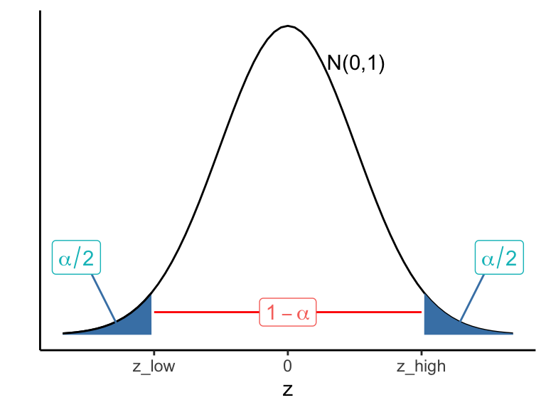
Figure 14.1: Finding z scores used to build a 2-sided confidence interval with desired confidence level
Similarly, a level \((1-\alpha)\) lower bound for \(\theta\) is \[\hat{\theta} - z_{\alpha}\cdot \sigma_{\hat{\theta}}\] (which defines the lower one-sided confidence interval \([\hat{\theta} - z_{\alpha}\cdot \sigma_{\hat{\theta}},\infty)\)) (see Figure 14.2).
A level \((1-\alpha)\) upper bound for \(\theta\) is \[\hat{\theta} + z_{\alpha}\cdot \sigma_{\hat{\theta}}\] (which defines the upper one-sided confidence interval \((-\infty,\hat{\theta}+z_{\alpha}\cdot \sigma_{\hat{\theta}}]\)) (see Figure 14.3). Note
- \(z_\alpha =\)
qnorm\((\alpha)\)
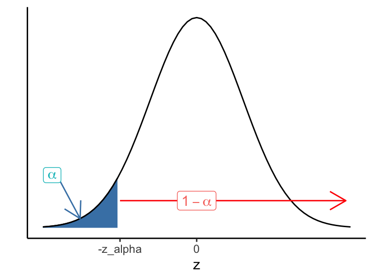
Figure 14.2: z scores corrsponding to lower 1-sided confidence interval
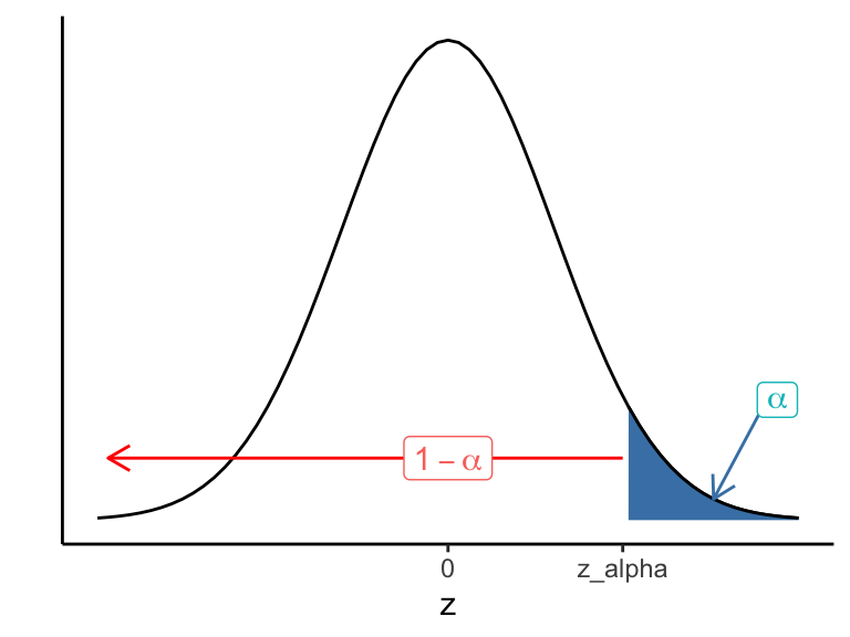
Figure 14.3: z scores corrsponding to upper 1-sided confidence interval
The scene outlined above applies to many situations, thanks to the Central Limit Theorem, including the four common scenarios mention in Chapter 13:
- 1 mean \(\mu,\) estimated with sample mean \(\overline{X},\)
- 1 proportion \(p,\) estimate with sample proportion \(\hat{p},\)
- difference of two means \(\mu_1-\mu_2,\) estimated with \(\overline{X_1}-\overline{X_2},\)
- difference of two proportions \(p_1-p_2,\) estimated with \(\hat{p_1}-\hat{p_2}\).
We summarize these confidence intervals here:
Common level \((1-\alpha)\) confidence intervals
- For \(\mu\): \[\overline{X} \pm z_{\alpha/2} \cdot \frac{\sigma}{\sqrt{n}}\]
- For \(p\): \[\hat{p} \pm z_{\alpha/2} \sqrt{\frac{p(1-p)}{n}}\]
- For \(\mu_1-\mu_2\): \[\left(\overline{X_1}-\overline{X_2}\right)\pm z_{\alpha/2} \frac{\sigma_1^2}{n_1} + \frac{\sigma_2^2}{n_2}\]
- For \(p_1-p_2\): \[\left(\hat{p}_1-\hat{p}_2\right)\pm z_{\alpha/2} \sqrt{\frac{p_1(1-p_1)}{n_1}+\frac{p_2(1-p_2)}{n_2}}\]
For large sample sizes (\(n\geq 30\) is often sufficient), \(S\) can be used for unknown \(\sigma\) in confidence intervals for means, and sample proportions \(\hat{p}\) can be used for unknown \(p\). For small sample sizes, when \(\sigma\) is unknown, we shall use \(T = \frac{\overline{X}-\mu}{S/\sqrt{n}}\) when estimating means, and we have the following confidence interval for \(\mu\):
For small sample sizes, when \(\sigma\) is unknown, we estimate \(\mu\) with \[\displaystyle \overline{X} \pm t_{\alpha/2} \cdot \frac{S}{\sqrt{n}}\]
Let’s work through several examples.
Example 14.4 Suppose we gather a sample of size \(n = 20\) from a \(N(\mu,2)\) population, and find \(\overline{x} = 16.3\). Find a 98% confidence interval for \(\mu\).
Here 98% confidence \(\leftrightarrow \alpha = 0.02,\) and \(z_{\alpha/2} = z_{.01}\) = qnorm(.99) = 2.326.
So our 98% confidence interval for the population mean \(\mu\) is \[\overline{x} \pm 2.326 \cdot \frac{2}{\sqrt{20}},\] or \[16.3 \pm 1.04,\] or \[15.26 \text{ to } 17.34.\]
Example 14.5 Suppose in this example we don’t know \(\sigma = 2,\) but in our sample of size 20 from \(N(\mu,\sigma),\) \(\overline{x} = 16.3\) and \(s = 2.13\). Find a 98% confidence interval for \(\mu\).
Using a sample standard deviation \(s\) in place of \(\sigma\) requires us to use \(t\) instead of \(z\). In particular, instead of using \(z_{.01} = 2.326,\) we must use \(t_{.01}(19),\) the value in the t(19) distribution that has 1% of the distribution greater than it.
So \(t_{.01}(19)\) = qt(.99,19) = 2.539. (This t-score will always be larger than the corresponding z-score, making the confidence interval wider than it would have been if we knew \(\sigma\).
Our confidence interval looks like: \[\overline{x} \pm 2.539 \cdot \frac{2.13}{\sqrt{20}},\] which simplifies to \[16.3 \pm 1.21,\] or, equivalently \[15.09 \text{ to } 17.51.\]
Example 14.6 In a poll of 500 likely voters, 260 say they support a particular local measure. Based on this sample, find a 90% confidence interval for \(p,\) the proportion of all likely voters in favor of this measure.
We use the large sample confidence interval for \(p\). From the data, \(n = 500,\) \(\hat{p} = 260/500 = .52,\) and for 90% confidence \(\alpha = 0.1,\) so \[z_{\alpha/2} = z_{.05} = 1.645,\]
(computed in R with qnorm(.95)). Now evaluate:
\[\begin{align*} \hat{p} \pm z_{\alpha/2} \sqrt{\frac{\hat{p}(1-\hat{p})}{n}} &= .52 \pm 1.645 \sqrt{\frac{(.52)(.48)}{500}}\\ &= .52 \pm .037\\ &= .483 \text{ to } .557. \end{align*}\]
It looks like it will be a close vote! We do not have convincing evidence, really, that \(p > .5\) since .5 lands inside the interval.
Example 14.7 (Angles of spider webs) The Handbook of Small Data Sets published in 1994 has lots of interesting, small data sets. Here’s one small data set:
Spider webs’ angles made with the vertical to the earth’s surface have a von Mises circular distribution with known mean direction, \(\mu,\) and \(\mu\) varies from species to species. For instance,
- Isoxya cicatricosa has \(\mu = 28.12^\circ,\) while
- Araneus rufipalpus has \(\mu = 15.66^\circ,\) obviously.
The question arose (in the article “Sequential analysis for angular data”, by Gadsden and Kanji, (1981), The Statistician, 30, 119-129) of which species had constructed the 10 webs whose angles were listed above in the vector X.
Treating the data as a simple random sample we can construct a 95% confidence interval for \(\mu\). Since the sample size is small, we use \(t_{\alpha/2},\) rather than \(z_{\alpha/2},\) where, here \(\alpha = .05\). Let’s crunch out the interval in R.
#summary statistics
n = length(X)
xbar = mean(X)
s = sd(X)
tstar = qt(.975,9) #we let tstar denote t_{alpha/2}
xbar + c(-1,1)*tstar*s/sqrt(n)
## [1] 13.67688 23.92312Based on the interval, which contains the known mean for Araneus rufipalpus, but not the known mean Isoxya cicatricosa, we have good evidence that these webs were made by the former type of spider.
Example 14.8 (Annual Snowfall in Buffalo, NY) Here’s another data set from the Handbook of Small Data Sets: The annual snowfall in Buffalo, NY (in inches) for the 63 years from 1910 to 1972.
##   year  snow
## 1 1910 126.4
## 2 1911  82.4
## 3 1912  78.1
## 4 1913  51.1
## 5 1914  90.9
Let’s find a 95% confidence interval for the mean annual snowfall in Buffalo, taking the above snowfall column as a simple random sample of annual snowfall. Here are the summary statistics:
For 95% confidence, \(\alpha = .05,\) and \(z_{\alpha/2} = z_{.025} \approx 1.96.\)
Since \(n\) is large, we use the confidence interval formula below with \(s\) plugged in for \(\sigma\):
\[\overline{x} \pm z_{\alpha/2} \cdot \frac{\sigma}{\sqrt{n}}\] and we arrive at the interval
## [1] 74.43965 86.15400Confidence Intervals for \(\mu_1-\mu_2\)
Suppose we have two samples from two populations: -an independent sample from population 1 which yields \(n_1,\) \(\overline{x}_1,\) \(s_1,\) and -an independent sample from population 1 which yields \(n_2,\) \(\overline{x}_2,\) \(s_2\). Moreover, the two samples are independent.
Recall, if Population 1 is \(N(\mu_1,\sigma_1)\) and Population 2 is \(N(\mu_2,\sigma_2\)), then a 95% confidence interval for \(\mu_1-\mu_2\) is \[\left(\overline{X_1}-\overline{X_2}\right)\pm z_{\alpha/2} \frac{\sigma_1^2}{n_1} + \frac{\sigma_2^2}{n_2}.\] If \(\sigma_1\) and \(\sigma_2\) are unknown, but \(n_1\) and \(n_2\) are fairly large, it is reasonable to replace \(\sigma_1\) and \(\sigma_2\) with \(s_1\) and \(s_2,\) respectively.
If \(n_1, n_2\) are small (\(\leq 30\)) it’s better to use a t-distribution.
Let’s consider the special case that \(\sigma_1\) and \(\sigma_2\) are unknown but equal. Letting \(\sigma^2\) denote this common value. In this case we consider the pooled sample variance: \[s_p^2 = \frac{(n_1-1)s_1^2 + (n_2-1)s_2^2}{n_1+n_2-2}\] as our (best) estimate of \(\sigma^2\). Then our level \((1-\alpha)\) confidence interval for \(\mu_1-\mu_2\) is \[\left(\overline{X_1}-\overline{X_2}\right)\pm t_{\alpha/2}S_p \sqrt{\frac{1}{n_1} + \frac{1}{n_2}},\] where \(t_{\alpha/2}\) live in a t-distribution with \(n_1+n_2-2\) degrees of freedom.
Example 14.9 The silver content (% Ag) of a number of Byzantine coins discovered in Cyprus was determined. Nine of the coins came from the first coinage of the reign of King Manuel, I, Comnenus (1143-1180); and 7 of the coins came from a coinage many years later.
The data
These data appear in The Handbook of Small Data Sets (p. 118), and are based on this article:
Hendy, M.F. and Charles J.A. (1970), The production techniques, silver content and circulation history of the twelfth-century Byzantine Trachy. Archaeonetry, 12. 13-21)
The question
Is there a significant difference in the silver content of coins minted early and late in Manuel’s reign?
Let’s conduct a small sample confidence interval for the difference in the two population means \(\mu_1 - \mu_2\) from the summary statistics:
| sample | n | xbar | s |
|---|---|---|---|
| 1 | 9 | 6.74 | 0.543 |
| 2 | 7 | 5.61 | 0.363 |
The pooled sample standard deviation is then \[s_p = \sqrt{\frac{8\cdot s_1^2 + 6 \cdot s_2^2}{14}} \approx .474,\]
and for 95% confidence we use \(t^*\) = qt(.975,14) = 2.145. With all these values we have the following 95% confidence interval for \(\mu_1 = \mu_2\): \[0.62 \text{ to } 1.64.\]
The entire interval lies above 0, so we have good evidence here of a difference between \(\mu_1\) and \(\mu_2\).
Was it reasonable in the previous example to assume the two populations have equal variance? Might differences in silver content in these two eras make it likely that other production differences existed as well (that might make variation in silver content from coin to coin also change)?
If \(\sigma_1^2\) and \(\sigma_2^2\) are unknown, sample sizes are samll, and its unreasonalbe to assume \(\sigma_1^2\) and \(\sigma_2^2\) are equal, one often sees the following (approximate) level \((1-\alpha)\) confidence interval for \(\mu_1 - \mu_2\):
\[\overline{X}_1 - \overline{X}_2 \pm t_{\alpha/2} \cdot \sqrt{\frac{s_1^2}{n_1}+\frac{s_2^2}{n_2}}\] where \(t_{\alpha/2}\) lives in a t-distribution with degrees of freedom equal to the minimum of \(n_1 - 1\) and \(n_2 - 1\).
So for the coin example, we would use \(t^*\) = qt(.975,6) = 2.447, giving us a wider confidence interval in the end:
\[0.574 \text{ to } 1.686,\] but still one that suggests a difference between \(\mu_1\) and \(\mu_2\).
Example 14.10 (Recent Buffalo Snowfall) With climate change, it may be unreasonable to assume the average annual snowfall now is the same as it was 100 years ago.
Let \(\mu_1\) denote the “old” mean average annual snowfall (and we assume the data from 1910 to 1972 is a random sample from the “old” population”), and \(\mu_2\) denots the “new” mean average annual snowfall in Buffalo (from which the annual snowfall from 2000 to 2021, found at buffalo.or/snow, is a random sample.) Do these data provide evidence that \(\mu_1 \neq \mu_2\)?
Here are the 2001-2022 data:
Y = c(158.7,132.4,111.3,100.9,109.1,78.2,88.9,103.8,100.2,74.1,111.8,
      36.7,58.8,129.9,112.9,55.1,76.1,112.3,118.8,69.2,77.2,97.4)
A 95% confidence interval for the difference \(\mu_X-\mu_Y\):
TODO
Example 14.11 (A one-sided confidence interval) The measures of the outside diameter \(x_i\) (in inches) for 9 grains of the same type:
Assume the distribution is normal. Is \(\mu \geq 2\)?
Let’s find a 1-sided lower bound 95% confidence interval for \(\mu,\) and see what that gets us.
Since \(n = 9\) is small and \(\sigma\) is unknown, we use the t-distribution.
Summary statistics:
- \(n = 9,\)
- \(\overline{x}\) =
mean(diam)= 1.9987. - \(s\) =
sd(diam)= 0.0122
For a lower bound 95% confidence interval, \(\alpha=.05\) and we use \[t_{\alpha} = t_{.05}(8) = qt(.95,8) = 1.86,\] and the lower 1-sided interval is
\[\begin{align*} (\overline{x}-t_{.05}(8)\cdot \frac{s}{\sqrt{n}},\infty) &= (1.9987 - 1.86\cdot\frac{0.0122}{\sqrt{9}},\infty) \\ &= (1.991,\infty) \end{align*}\]
This confidence interval does not convince me that \(\mu \geq 2\). (If the interval had been something like \([2.01,\infty),\) then I would be more convinced since we’re confident that \(\mu\) is within the confidence interval, but with the interval \([1.991,\infty),\) best we can say is we’re confident \(\mu \geq 1.99\).