9 Continuous Random Variables

We now turn our attention to continuous random variables.

9.1 Distribution Functions

Definition 9.1 (Distribution Function of a Random Variable) Let \(X\) be a random variable. The distribution function of \(X,\) denoted \(F(x),\) is the function defined on all real numbers \(x\) such that \[F(x) = P(X \leq x).\]

Example 9.1 Suppose \(X\) is the discrete random variable given by density function \[ \begin{array}{c|c|c|c|c} x & 0 & 1 & 2 & 3 \\ \hline p(x) & 1/8 & 3/8 & 3/8 & 1/8 \end{array} \] Note \(F(-2.7) = P(X \leq -2.7) = 0,\) and \(F(1.3) = P(X \leq 1.3) = 1/8 + 3/8 = 4/8\) (since the only \(X\) values less than or equal to 1.3 with positive probability are \(X=0\) or \(X=1\)).

The distribution function for \(X\) is the following step function:

\[ F(x)= \begin{cases} 0 &\text{ if }x < 0 \\ 1/8 &\text{ if } 0 \leq x < 1 \\ 4/8 &\text{ if } 1 \leq x < 2 \\ 7/8 &\text{ if } 2 \leq x < 3 \\ 1 &\text{ if } x \geq 3 \end{cases} \]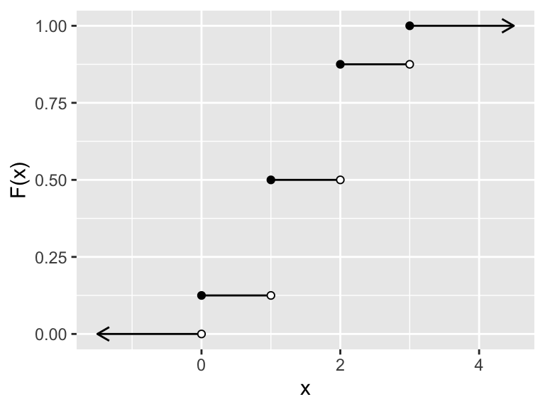

Figure 9.1: Distribution function for X

Observe that this function \(F(x)\) is defined for all \(-\infty < x < \infty\) (check out those arrows :)). The jumps in the graph indicate that the function \(F\) is not continuous, and the points of discontinuity occur exactly at the values of \(X\) in the probability table for \(X\).

Theorem 9.1 (Properties of any distribution function) If \(F(x)\) is a distribution function, then

1. \(\displaystyle \lim_{x \to -\infty} F(x) = 0\);
2. \(F\) is non-decreasing. That is, if \(x_1 \leq x_2\) then \(F(x_1) \leq F(x_2)\); and
3. \(\displaystyle \lim_{x \to \infty} F(x) = 1\).

Definition 9.2 (Continuous Random Variable) A random variable is called a continuous random variable if its distribution function \(F\) is continuous for all \(x\).

So the distribution function for any continuous random variable has the following sort of look, descriptively (as in Figure 9.2):

• it is continuous,
• its domain is \((-\infty,\infty)\)
• as \(x\) progresses away from \(-\infty\) toward \(\infty,\) the values of \(F(x)\) rise from 0 to 1, never decreasing along the way.

Definition 9.3 Let \(F\) be the distribution for a continuous random variable \(X\). Then the derivative of \(F,\) wherever it exists is called the probability density function for \(X\). When continuous \(X\) has a probability density function, we usually denote it as \(f(x)\).

The density function \(f(x)\) is a theoretical curve for the frequency distribution of a population of measurements. We’ll look at examples shortly.

Theorem 9.2 (Properties of a density function) If \(f(x)\) is a density function for a continuous random variable \(X,\) then

1. \(f(x) \geq 0\) for all \(x,\) and
2. \(\displaystyle \int_{-\infty}^{\infty} f(x)~dx = 1\).

Sketch of Proof:

For a) Recall \(f(x) = F^\prime(x)\). One feature of any distribution function is that it is never decreasing, so its slope (derivative) is never negative. Since \(f(x)\) gives the slope of \(F,\) \(f(x) \geq 0\).

For b) \(F\) is the antiderivative of \(f,\) which is useful to know when we integrate \(f\). Also, \(\displaystyle \int_{-\infty}^{\infty} f(x)~dx\) is an improper integral, which we can tackle by splitting it into two integrals, assuming each of these new integrals converges:

\[\begin{align*} \int_{-\infty}^{\infty} f(x)~dx &= \int_{-\infty}^{0} f(x)~dx + \int_{0}^{\infty} f(x)~dx \\ &= \lim_{a \to -\infty} \int_a^0 f(x)~dx + \lim_{b \to \infty} \int_0^b f(x)~dx \\ &= \lim_{a \to -\infty} \left[F(0)-F(a)\right] + \lim_{b \to \infty} \left[F(b)-F(0)\right] \\ &= (F(0)-0) + (1 - F(0)) & \text{ by limit properties of } F \\ &= 1. \end{align*}\]

Example 9.2 Consider distribution function \(F\) pictured below, where \(c > 0\) is a fixed constant.

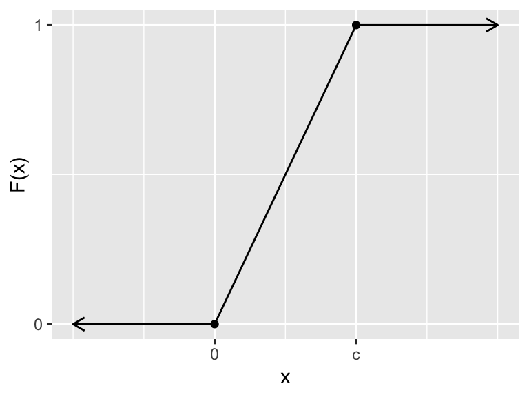
Figure 9.2: Piece-wise linear distribution function

This function is piece-wise linear, continuous, and it is differentiable everywhere except the sharp corners at \(x = 0\) and \(x = c\). At any other point, \(f(x) = F^\prime(x)\) equals the slope of the segment running through the point \((x,F(X))\).

So the probability density function for this random variable is \[ f(x)= \begin{cases} 0 &\text{ if }x < 0 \\ 1/c &\text{ if } 0 < x < c \\ 0 &\text{ if } x > c, \end{cases} \] and the graph of \(f\) looks like this:

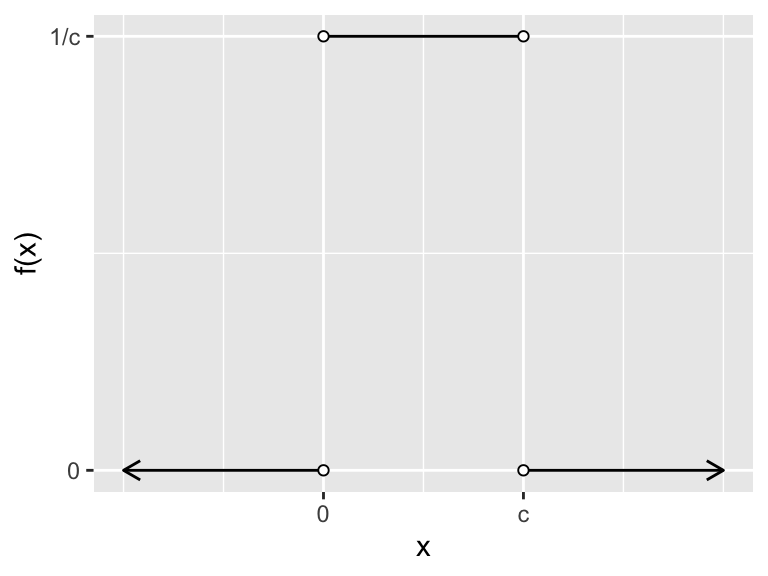
Figure 9.3: probability density function for X

Note that \(f(x) \geq 0\) for all \(x\). Also, \[\int_{-\infty}^{\infty} f(x)~dx = \int_0^c f(x)~dx\] (we only have to integrate over intervals in which \(f(x) > 0\)), and this later integral is the area of a rectangle of width \(c\) and height \(1/c,\) so it has area 1. Thus, we have a valid pdf!

Example 9.3 Find the value of \(k\) that makes the following function a valid pdf. \[ f(x)= \begin{cases} kx^8 &\text{ if }0 \leq x \leq 1 \\ 0 &\text{ else.} \end{cases} \] We need \(k \geq 0\) os that \(f(x) \geq 0\) for all \(x\). We also need \[1 = \int_{-\infty}^\infty f(x)~dx = \int_0^1 kx^8~dx = \frac{k}{9}x^9 ~\biggr|_0^1.\] It follows that \(k = 9\).

Definition 9.4 (Quantiles) Let \(X\) denote a random variable. If \(0 < p < 1,\) the \(p\)th quantile of \(X,\) denoted \(\phi_p,\) is the smallest value such that \(F(\phi_p) \geq p\). If \(X\) is continuous, \(\phi_p\) is the smallest value such that \(F(\phi_p) = p\).

Some special quantiles:

• \(\phi_.25,\) denoted \(Q1,\) is called the first quartile,
• \(\phi_.5,\) denoted \(M,\) is called the median of the random variable,
• \(\phi_.75,\) denoted \(Q3,\) is called the third quartile

Theorem 9.3 If \(X\) is a continuous random variable with density function \(f,\) then for any real numbers \(a < b,\) \[P(a \leq X \leq b) = \int_a^b f(x)~dx.\]

Proof Idea: The distribution function \(F\) is an antiderivative of the density function \(f,\) so using the Fundamental Theorem of Calculus,

\[\begin{align*} \int_a^b f(x)~dx &= F(b) - F(a) \\ &= P(X\leq b) - P(X \leq a) \\ &= P(a < X \leq b) &\text{ since } a < b\\ &= P(a \leq X \leq b) &\text{ since } P(X = a) = 0 \end{align*}\]

Note: For any continuous random variable \(X,\) and \(a < b,\)

\[P(a < X < b) = P(a \leq X < b) = P(a < X \leq b) = P(a \leq X \leq B)\] since \(P(X = c) = 0\) for any real number \(c\).

Example 9.4 (A quadratic density function) Suppose \(X\) has density function \[ f(x)= \begin{cases} \frac{3}{8}x^2 &\text{ if }0 \leq x \leq 2 \\ 0 &\text{ else.} \end{cases} \]

Wait! Is this actually a valid density function?

1. Ok, yes, \(f(x) \geq 0\) for all \(x\).
2. And…

\[\begin{align*} \int_{-\infty}^{\infty} f(x) ~dx &= \int_0^2 \frac{3}{8} x^2~dx \\ &= \frac{1}{8} x^3 \Big|_0^2 \\ &= 1. \end{align*}\]

Ok, now to the question: Find \(P(1 \leq X \leq 2)\):

\[\begin{align*} P(1 \leq X \leq 2) &= \int_1^2 \frac{3}{8} x^2~dx \\ &= \frac{1}{8} x^3 ~\biggr|_1^2 \\ &= 1 - \frac{1}{8} \\ &= \frac{7}{8}. \end{align*}\]

Even though \(X\) can take any value between 0 and 2, the probability is 7/8 that \(X\) will be between 1 and 2. Most of the area under the density curve is at the high end of the \(X\) range:

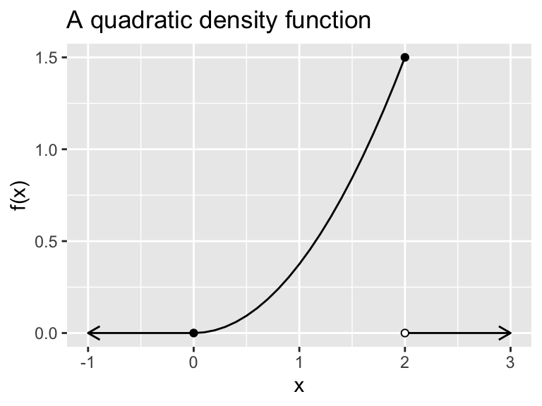
Figure 9.4: A quadratic density function

Example 9.5 Suppose \(X\) has density function \[ f(x)= \begin{cases} 0 &\text{ if } x < 1 \\ \frac{1}{x^2} &\text{ if } x \geq 1. \end{cases} \]

a) Check that this gives a valid density function:

\[\begin{align*} \int_{-\infty}^{\infty} f(x)~dx &= \int_1^\infty x^{-2}~dx \\ &= \lim_{b \to \infty} \left[\int_1^b x^{-2}~dx \right] \\ &= \lim_{b \to \infty} \left[ -\frac{1}{x} \biggr|_1^b \right]\\ &= \lim_{b \to \infty} \left[ -\frac{1}{b}+1\right]\\ &= 1. \end{align*}\] The limit equals 1 in the end since \(1/b \to 0\) as \(b \to \infty\).

b) Find \(F(x),\) the cumulative probability distribution function.

By definition, for any real number \(x,\) \[F(x) = \int_{-\infty}^x f(t)~dt,\] which, of course, gives the area under \(f\) over the interval \((-\infty, x]\). Since \(f\) is piece-wise defined, the integrand used in the integral to evaluate \(F\) depends on the bounds of the integral.

\[ F(x)= \begin{cases} \displaystyle\int_{-\infty}^x 0 ~dt &\text{ if } x < 1 \\ \displaystyle\int_{-\infty}^1 0 ~dt + \displaystyle\int_{1}^x \frac{1}{t^2} ~dt&\text{ if } x \geq 1. \end{cases} \] We leave it to the reader to integrate these expressions to obtain \[ F(x)= \begin{cases} 0 &\text{ if } x < 1 \\ \displaystyle 1 - \frac{1}{x} &\text{ if } x \geq 1. \end{cases} \]

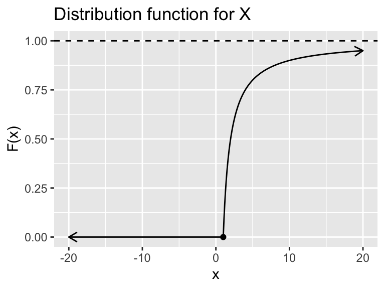
Figure 9.5: Distribution function for X

c) Find \(P(1 < X < 3).\)

Well, \[P(1 < X < 3) = \int_1^3 f(x)~dx = F(3)-F(1),\] by the Fundamental Theorem of Calculus (FTC), so \[P(1 < X < 3) = (1 - 1/3) - (1 - 1/1) = 2/3.\]

9.2 Expected Value for Continuous Random Variables

Definition 9.5 If \(X\) is a continuous random variable with probability density function \(f(x),\) then the expected value of \(X\), denoted \(E(X),\) is \[E(X) = \int_{-\infty}^\infty x \cdot f(x)~dx,\] provided this integral exists. The expected value \(E(X)\) is also called the mean of \(X\), and is often denoted as \(\mu_X,\) or \(\mu\) if the random variable \(X\) is understood.

The expected value of the function \(g(X)\) of \(X\) is \[E(g(X)) = \int_{-\infty}^\infty g(x) \cdot f(x)~dx,\] provided this integral exists.

The variance of \(X\) is \[V(X) = E((X-\mu_X)^2),\] provided this integral exists.

As in the discrete case, one can show \(V(X) = E(X^2)-E(X)^2,\) a working formula for variance which is sometimes easier to use to calculate variance.

Example 9.6

Find \(E(X)\) and \(V(X)\) where \(X\) is the continuous random variable from Example 9.4.

Recall \(X\) has density function \(\displaystyle f(x) = 3x^2/8\) for \(0 \leq x \leq 2\).

Expected Value: \[\begin{align*} E(X) &= \int_0^2 x \cdot 3x^2/8~dx \\ &= \frac{3}{8} \int_0^2 x^3~dx \\ &= \frac{3}{8}\frac{1}{4}x^4 ~\biggr|_0^2 \\ &= \frac{3}{2}. \end{align*}\]

Variance: We first find \(E(X^2)\): \[\begin{align*} E(X^2) &= \int_0^2 x^2 \cdot 3x^2/8~dx \\ &= \frac{3}{8} \int_0^2 x^4~dx \\ &= \frac{3}{8}\frac{1}{5}x^5 ~\biggr|_0^2 \\ &= \frac{12}{5}. \end{align*}\]

Then, \[\begin{align*} V(X) &= E(X^2) - E(X)^2 \\ &= (12/5) - (3/2)^2\\ &= 0.15. \end{align*}\]

The properties of expected value that held for discrete random variables also hold for continuous random variables.

Theorem 9.4 Suppose \(X\) is a continuous random variable, \(c \in \mathbb{R}\) is a constant, and \(g,\) \(g_1,\) and \(g_2\) are functions of \(X\).

1. \(E(c) = c\).
2. \(E(c\cdot g(X))= cE(g(X))\).
3. \(E(g_1(X) \pm g_2(X)) = E(g_1(X)\pm g_2(X))\).

These results follow immediately from properties of integration. For instance, to prove property 1 we observe that for constant \(c,\) \[E(c) = \int_{-\infty}^\infty c\cdot f(x)~ dx = c \int_{-\infty}^\infty f(x)~ dx,\] and the integral in the last expression equals 1 by definition of a valid probability density function.

Theorem 9.5 Let \(X\) be a random variable (discrete or continuous) with \(E(X) = \mu\) and \(V(X) = \sigma^2,\) and let \(a, b\) be constants. Then

1. \(\displaystyle E(aX + b) = aE(X) + b = a \mu + b.\)
2. \(\displaystyle V(aX + b) = a^2V(X) = a^2 \sigma^2.\)

Proof.

1. This result follows immediately from properties of expected value (Theorems 9.4 and 9.4).

2. Let \(Y = aX + b\). Then (a) says that \(E(Y) = a \mu + b,\) so \[\begin{align*} V(Y) &= E((Y-(a\mu + b))^2) \\ &= E\left(((aX+b)-(a\mu + b))^2\right)\\ &= E\left((aX-a\mu)^2\right)\\ &= a^2 E\left((X-\mu)^2\right) \end{align*}\] But \(E\left((X-\mu)^2\right)=V(X)\) by the definition of variance, so the result follows.

Example 9.7 (Ore Sample Impurities) For certain ore samples, the proportion \(X\) of impurities per sample is a random variable with density function \[ f(x)= \begin{cases} 1.5x^2 + x &\text{ if }0 \leq x \leq 1 \\ 0 &\text{ else. } \end{cases} \] The dollar value of each sample is \(W = 5 - 0.5X\).

Find the mean, variance, and standard deviation of \(W\).

First, let’s consider the variable \(X\) itself.

\[\begin{align*} E(X) &= \int_0^1 x \cdot (1.5x^2 + x)~dx \\ &= \int_0^1 1.5x^3 + x^2~dx \\ &= \frac{1.5}{4}x^4 + \frac{1}{3} x^3 ~\biggr|_0^1 \\ &= \frac{17}{24}. \end{align*}\]

Also, \[\begin{align*} E(X^2) &= \int_0^1 x^2 \cdot (1.5x^2 + x)~dx \\ &= \int_0^1 1.5x^4 + x^3~dx \\ &= \frac{1.5}{5}x^5 + \frac{1}{4} x^4 ~\biggr|_0^1 \\ &= \frac{11}{20}. \end{align*}\]

Thus, \(V(X) = (11/20)-(17/24)^2 \approx 0.0483.\)

Then, by Theorem 9.5,

\[E(W) = E(5 - 0.5X) = 5 - 0.5E(X) = 5 - 0.5\cdot (17/24) = 4.65,\] and \[V(W) = V(5 - 0.5X) = 0.25V(X) \approx 0.012,\] so that the standard deviation is \(\sigma = \sqrt{V(W)} ~\approx 0.11\) (about 11 cents).