13 Estimation
The Scene: We want to estimate some parameter \(\theta\) of a population by gathering and analyzing an independent random sample drawn from the population.
13.1 Unbiased Estimators
Definition 13.1 A statistic is any function of a random sample \(X_1, X_2, \ldots X_n\) drawn from a population.
Definition 13.2 A statistic \(\hat{\theta}\) based on a random sample \(X_1, X_2, \ldots X_n\) is an unbiased estimator of the population parameter \(\theta\) if \(E(\hat{\theta}) = \theta\).
The bias of \(\hat{\theta}_n\) is \(B(\hat{\theta}) = E(\hat{\theta})-\theta\).
The mean square error of \(\hat{\theta}_n\) is MSE\((\hat{\theta}) = E[(\hat{\theta}-\theta)^2]\).
A good estimator for the parameter \(\theta\) is a statistic \(\hat{\theta}\) that is unbiased with variance as small as possible. These features of \(\hat{\theta}\) would ensure that for any random sample you happen to gather, the value \(\hat{\theta}\) you compute from the data is likely to be close to \(\theta\) (or at least likelier to be close to \(\theta\) than some other statistic).
Example 13.1 (Two unbiased estimators for the upper bound of a uniform distribution) Suppose \(X_1, X_2, \ldots, X_n\) is an independent random sample drawn from a uniform distribution \(U(0,\theta),\) where \(\theta\) is unknown. So each \(X_i\) is a random real number between 0 and \(\theta\).
How can we estimate the unknown parameter \(\theta\) from the data?
First estimator: Create an estimator from the sample mean: \[\overline{X} = \frac{1}{n}\sum_{i = 1}^n X_i.\]
By properties of expected value, \[\begin{align*} E(\overline{X}) &= \frac{1}{n}\sum_{i = 1}^n E(X_i) \\ &= \frac{1}{n}\sum_{i = 1}^n \frac{\theta}{2} \end{align*}\] since each \(X_i\) is \(U(0,\theta),\) so \(E(X_i) = \frac{0 + \theta}{2}\).
It follows that \[E(\overline{X}) = \frac{1}{n} \cdot n \cdot \frac{\theta}{2} = \frac{\theta}{2}.\]
Since \(E(\overline{X}) \neq \theta,\) the sample mean \(\overline{X}\) is not an unbiased estimator for \(\theta\). This makes sense. We shouldn’t expect the average of the random numbers to be a good estimate of the upper bound of the interval from which the numbers were picked.
However, \(E(\overline{X})\) does equal a constant multiple of \(\theta,\) which means we can easily adjust \(\overline{X}\) to a statistic that is an unbiased estimator for \(\theta\):
\[\hat{\theta}_1 = 2\overline{X} \tag{unbiased estimator 1}\] Second Estimator: Create an estimator from the maximum value of the data, since this max is “closest” to \(\theta\) of all the data points.
Let \(Y = \max\{X_1, X_2, \ldots, X_n\}.\) We prove below in 13.2 that \[E(Y) = \frac{n}{n+1}\theta.\] Assuming that for now, we can say that \[\hat{\theta}_2 = \frac{n+1}{n}\cdot Y \tag{unbiased estimator 2}\] is also an unbiased estimator for \(\theta\).
Let’s see how these different estimators do for a particular random sample generated in R.
theta = 20 # we pretend we don't know this parameter
n = 10 # the size of the sample
X = runif(n,0,theta) # generate the random sample
est_1 = 2*mean(X)
est_2 = (n+1)/n*max(X)
print(round(X,2))
## [1] 13.47 13.74 12.24 8.86 8.65 12.61 5.67 5.69 9.13 8.77For this single sample the estimators takes on these values:
- Estimator 1: \(\hat{\theta}_1\) = 19.8
- Estimator 2: \(\hat{\theta}_2\) = 15.1.
The fact that both estimators are unbiased means that in the long run, the average of all the \(\hat{\theta}_1\) estimates would approach \(\theta,\) and the same is true for the average of the \(\hat{\theta}_2\) estimates.
So, they’re both good estimaors of \(\theta\) in that regard. What makes one estimator better is if the variation of the estimates obtained from repeated sampling is smaller for one than the other.
Let’s simulate drawing 1000 different samples of size \(n = 10,\) recording the distribution of values taken by the estimates \(\theta_1\) and \(\theta_2,\) and seeing which distribution has smaller variance.
theta = 20;n = 10 # the size of the sample in each trial
trials = 1000 # number of times we take a sample of size n
dist_1 = c() # records estimator 1 values
dist_2 = c() # records estimator 2 values
# run the trials
for (i in 1:trials){
  X = runif(n,0,theta) # generate the random sample
  dist_1[i] = 2*mean(X)
  dist_2[i] = (n+1)/n*max(X)
}
# create data frame of results for ggplot
df = rbind(data.frame(estimator = "1",value = dist_1),
           data.frame(estimator = "2",value = dist_2))
# plot
ggplot(df)+
  geom_density(aes(x=value,fill=estimator),alpha = .4)+
  theme_get()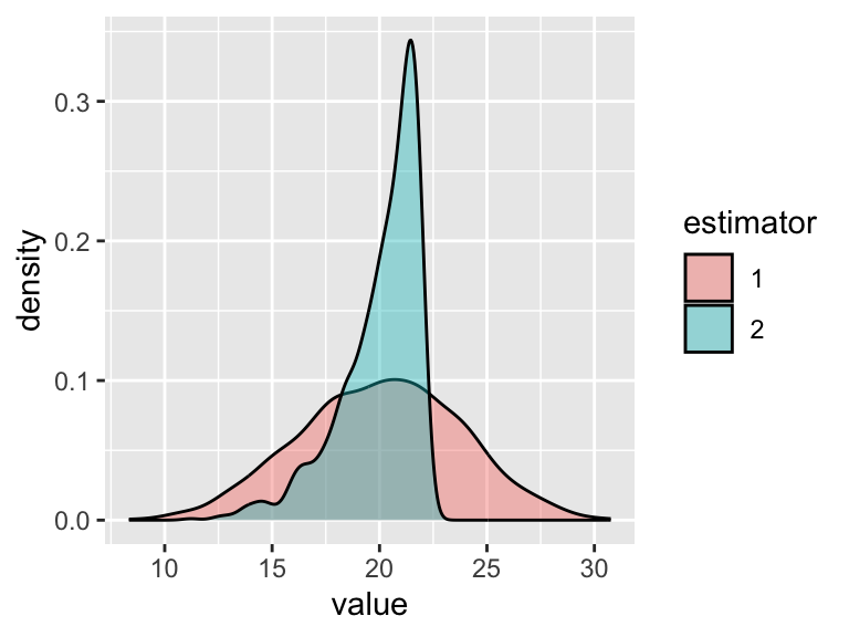
Figure 13.1: Sampling distributions for two unbiased estimators
Both estimators have average value near 20. In fact,
mean(dist_1)- = 19.8mean(dist_2)= 20.03.
But the estimator 2 distribution has visibly smaller variance. Indeed,
sd(dist_1)= 3.65sd(dist_2)= 1.86.
It appears that the better estimator here is the one derived from the maximum value of the data as opposed to the mean of the data.
13.2 Order Statistics
If \(X_1, X_2, \ldots, X_n\) is a sample drawn from a distribution with density function \(f_X(x),\) let \[Y = \text{max}\{X_1, X_2, \ldots, X_n\}.\] We can deduce the density function for \(Y\) by first writing down the distribution function. For any real number \(y,\) \[\begin{align*} F_Y(y) &= P(Y \leq y) \\ &= P(\text{all }X_i \leq y) \\ &= P(X_1 \leq y, X_2 \leq y, \ldots, X_n \leq y) \\ &= \left[F_X(y)\right]^n. \end{align*}\] We differentiate \(F_Y\) with the chain rule to find \(f_Y\): Thus, \[f_Y = n\left[F_X(y)\right]^{n-1}\cdot f_X(y). \tag{density for the max of sample}\] For \(X\) is \(U(0,\theta)\) as in the previous example, \(f_X(x) = 1/\theta,\) and \(F_X(x) = x/\theta,\) for \(0 \leq x \leq \theta\). So, the density function for \(Y = \text{max}(X_i),\) where \(X_i\) is \(U(0,\theta)\) is \[\begin{align*} f_Y(y) &= n \left[\frac{y}{\theta}\right]^{n-1} \cdot \frac{1}{\theta}\\ &= \frac{n}{\theta^n}y^{n-1}, \end{align*}\] for \(0 \leq y \leq \theta,\) and \[E(Y) = \int_0^\theta y \cdot \frac{n}{\theta^n}y^{n-1}~dy = \cdots = \frac{n}{n+1}\theta,\] giving us the result we assumed when defining estimator 2 in the previous example.
In the homework you derive the density function for the minimum of a random sample.
13.3 Common Unbiased Estimators
We have seen the following strategy for finding unbiased estimators: Try a simple estimator (e.g., \(\overline{X}\) or max\((X_i)\)) and tweak it so that it becomes unbiased.
13.3.1 Estimating \(\mu,\) a population mean
If \(X_1, X_2, \ldots, X_n\) is a sample drawn from a distribution with mean \(\mu\) and standard deviation \(\sigma\) we have seen that the sample mean \(\overline{X}\) has \(E(\overline{X}) = \mu\) and standard deviation \(\sigma/\sqrt{n}\). That is,
\(\overline{X}\) is an unbiased estimator for \(\mu,\) and its standard deviation is \(\sigma/\sqrt{n}\).
13.3.2 Estimating \(p,\) a population proportion
If \(X_1, X_2, \ldots, X_n\) is a sample drawn from a \(b(1,n)\) distribution (Bernoulli trial!) and \(X = X_1 + X_2 + \cdots + X_n\) equals the number of successes in \(n\) trials, then we have seen that \(\hat{p} = X/n\) has \(E(\hat{p}) = p\) and standard deviation \(\displaystyle\sqrt{\frac{p(1-p)}{n}}\). That is,
\(\hat{p}\) is an unbiased estimator for \(p,\) and its standard deviation is \(\displaystyle\sqrt{\frac{p(1-p)}{n}}\).
Example 13.2 In a sample of 65 Linfield students, 24 are first-generation students. Estimate \(p,\) the proportion of all Linfield students that are first-generation, and place a 2 standard deviation bound on the error of estimation.
From our sample, our point estimate for \(p\) is \(\hat{p} = 24/65 \approx .369.\) We know by the CLT that \[\hat{p} \sim N(p, \sqrt{p(1-p)/n}),\] and in a normal distribution, about 95% of the distribution is within two standard deviations of the mean. In other words, \[P\left(~|\hat{p}-p|<2\cdot\sqrt{p(1-p)/n}~\right) \approx 0.95.\] Now we don’t know \(p\) (in fact, we’re trying to estimate it!), so we can’t know the value of the standard deviation \(\sqrt{p(1-p)/n}.\) However, for large \(n,\) the expression \(\sqrt{x(1-x)/n}\) doesn’t change much for nearby inputs, except when the inputs are close to 0 or 1 (try it!). In other words, we can reasonably expect \[\sqrt{\hat{p}(1-\hat{p})/n} ~\approx \sqrt{p(1-p)/n},\] in which case we can estimate that \[P\left(~|\hat{p}-p|<2\cdot\sqrt{\hat{p}(1-\hat{p})/n}~\right) \approx 0.95.\] In this problem \(\hat{p} \approx .37,\) so \(2 \cdot \sqrt{p(1-p)/n} \approx 0.12,\) so we can say that \[|.37-p| < 0.12\] with probability about .95, and that \[ .25 < p < .49\] gives a two standard deviation bound on the error of estimation.
13.3.3 Estimating \(\mu_1 - \mu_2,\) the difference of two population means
Suppose we have two independent random samples drawn from distinct normal distributions.
- \(X_1, \ldots, X_{n_1} \sim N(\mu_1,\sigma_1)\)
- \(Y_1, \ldots, Y_{n_2} \sim N(\mu_2, \sigma_2)\)
Let \(\overline{X}\) and \(\overline{Y}\) denote the respective sample means, and consider the point estimate \(\overline{X}-\overline{Y}\) of \(\mu_1-\mu_2\). Since \(\overline{X}-\overline{Y}\) is a linear combination of normal random variables, we can show \(\overline{X}-\overline{Y}\) is itself normal, with
- mean = \(E(\overline{X}-\overline{Y}) = E(\overline{X})-E(\overline{Y}) = \mu_1 - \mu_2\)
- variance = \(V(\overline{X}-\overline{Y}) = V(\overline{X})+V(\overline{Y}) = \frac{\sigma_1^2}{n_1} + \frac{\sigma_2^2}{n_2}\).
So \(\overline{X}-\overline{Y}\) is an unbiased estimator for \(\mu_1 - \mu_2\) with standard deviation equal to \(\displaystyle\sqrt{\sigma_1^2/n_1 + \sigma_2^2/n_2}.\)
13.3.4 Estimating \(p_1 - p_2,\) the difference of two population proportions
An unbiased estimator for \(p_1-p_2\) is \(\hat{p}_1-\hat{p}_2,\) where \(\hat{p}_i\) equals the sample proportion from a sample of size \(n_i\) drawn from population \(i\) (which has population proportion \(p_i\)).
One can show that the point estimate \(\hat{p}_1 - \hat{p}_2\) is approximately normal with mean \(p_1-p_2\) and standard deviation \(\displaystyle \sqrt{\frac{p_1(1-p_1)}{n_1}+\frac{p_2(1-p_2)}{n_2}}\) for reasonably sized samples (more on this later). For now lets consider an example.
Example 13.3 (Two Large Buckets) Each of two large buckets is full of two types of marbles, orange and green. Let \(p_i\) denote the proportion of orange marbles in bucket \(i\) (\(i = 1,2\)).
Estimate \(p_1-p_2,\) and place a 2 standard deviation bound on the error of estimation.
- Sample 1: \(n_1 = 120\) marbles from bucket 1, of which 45 are orange, so \(\hat{p}_1 = .375\)
- Sample 2: \(n_2 = 80\) marbles from bucket 2, of which 36 are orange, so \(\hat{p}_2 = .45\).
Point estimate: \[\hat{p}_1 - \hat{p}_2 = -.075.\] Also, it is reasonable to assume that the sampling distribution for \(\hat{p}_1-\hat{p}_2\) is approximately \[N\left(p_1-p_2, \sqrt{\frac{\hat{p}_1(1-\hat{p}_1)}{n_1}+\frac{\hat{p}_2(1-\hat{p}_2)}{n_2}}\right)\] (again, plugging in \(\hat{p}_i\) for \(p_i\) in the standard deviation is “ok” for larger sample sizes and values of \(\hat{p}_i\) not too close to 0 or 1.).
For a normal distribution, about 95% of the distribution falls within 2 standard deviations of the mean, so \[P\left(|(\hat{p}_1-\hat{p}_2)-(p_1-p_2)|< c\right)\approx .95,\] where \[c = 2\cdot \sqrt{\frac{\hat{p}_1(1-\hat{p}_1)}{n_1}+\frac{\hat{p}_2(1-\hat{p}_2)}{n_2}}.\]
So, we can say that \[\hat{p}_1-\hat{p}_2 - c < p_1 - p_2 < \hat{p}_1-\hat{p}_2 + c\] with probability about .95. Plugging in numbers in this example, we obtain the interval \[-0.217 < p_1 - p_2 < 0.067.\]
Hmm… this interval contains 0. While the sample proportions here are such that we may suspect the second bucket has a higher proportion of orange marbles, when we take into account the error of estimation due to sampling variability, our samples do not provide overwhelming evidence that the buckets have different proportions of orange marbles.