Tips for Getting Started with RStudio in MATH 140
1. Install R and RStudio
You will first need to download and install both R and RStudio (Desktop version) on your computer. R and RStudio are separate installations. R is a programming language that is convenient to use in statistics. RStudio is a user-friendly interface that makes using R easier.
The following installation instructions are taken from Section 1.1.1 of ModernDive, a well-written, freely available text.
- You must do this first: Download and install R by going to https://cloud.r-project.org
- If you are a Windows user: Click on “Download R for Windows”, then click on “base”, then click on the Download link.
- If you are macOS user: Click on “Download R for (Mac) OS X”, then under “Latest release:” click on R-X.X.X.pkg, where R-X.X.X is the version number.
- If you are a Linux user: Click on “Download R for Linux” and choose your distribution for more information on installing R for your setup.
- You must do this second: Download and install RStudio at https://www.rstudio.com/products/rstudio/download/.
- Scroll down to “Installers for Supported Platforms” near the bottom of the page.
- Click on the download link corresponding to your computer’s operating system.
I recommend reading all of section 1.1.1 in ModernDive as you get started with RStudio.
2. Orient yourself in RStudio
The RStudio interface has four window panes (the red division lines appearing in the image below were added for dramatic effect).

Here’s a quick introduction to each of these panes.
Upper Left: Source Editor
Files meant to run in RStudio, such as scripts or
Rmarkdown files, will appear here. In the screenshot above, the
source pane has one script loaded, called governors.R, which is
a file that helps us investigate a data set related to the current
governors of the 50 U.S. States.
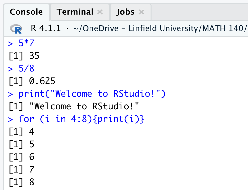
Lower Left: Console
The console pane has a command line prompt > at which we
can enter commands. We can use RStudio as a calculator, we can ask it to
print statements, and we can do some programming, and other cool
things:
Pro Tip: At the console prompt click the up and down arrows to scroll through previously entered commands.
Upper Right: Workspace Browser
The workspace browser has several tabs. The two we will use most are
these:
- Environment tab gives information about the data frames, variables, and functions that you’ve loaded into your RStudio session.
- History tab. This tab records all the commands you’ve run. This history can be helpful if you’re wondering how you did a certain thing a while back… .
You can clear your workspace browser by clicking on the broom icon near the upper right corner of the workspace browser pane.
In the screenshot above, the Environment tab appears in the
Workspace, and shows two items, a dataframe called gov, and
a vector called party_colors, used to choose the red and
blue colors appearing in plots. The data frame gov has has
50 rows (observations), one for each state, and 11 columns (variables),
containing information like the governor’s name, age at inauguration,
political party.
Lower Right: Plots and Files The lower right pane in RStudio has several much-used tabs.
- The Files tab shows the file system in your computer.
- The Plots tab is where your beautiful graphics will
appear
- The Help tab is super helpful! If you want to learn more about a command or a built-in data set, the help tab is there - and there are usually built-in examples to demonstrate ideas.
- The Packages tab is in this pane as well. We talk about packages below.
In the screenshot the Plots tab is open, showing side-by-side boxplots of Governor ages by political party. Incidentally, the code for producing this plot is visible in the Source pane of this screenshot.
3. Use a Folder System
Organize a folder system on your computer to help you keep track of your files and data sets. Here’s my suggestion:
Create a folder dedicated to this class on your computer, perhaps the desktop, with a descriptive name, say “math140”.
Create a subfolder in your “math140” folder for each RStudio project you work on. For instance, you might create a folder called “lab1” in your “math140” folder ahead of our first lab.
4. Create Projects
Project files in Rstudio help you organize your work, and connect
RStudio with your computer’s file system.
By the end of the term your “math140” folder may have 5 or 6 different
subfolders. One for each lab, one for your term project, one for top
secret data analysis - who knows. If you attach a project file to each
of these subfolders then it is easy in RStudio to shift between these
projects.
To create a project, follow these steps:
Open RStudio
Create a project from the File menu (File -> New Project), or by moving the cursor to the upper-right corner of your RStudio window and selecting Project > New Project.
Select Existing Directory in the pop-up menu.
Click Browse and navigate to where you created the lab1 folder. Select this folder and then click Create Project.
Your R project has now been created. Note that in the upper right-hand corner, the program indicates that you are working on the project named lab1. In the future you can click on this spot in the upper right corner to change the project you want to work on or create a new one.
Note also that if you click on the Files tab in the lower right pane in RStudio, you can access the file system on your computer. By default, RStudio will show the contents of your current project folder
In addition to the project file itself, my mature project folders often contain three types of files:
- R script files (discussed below)
- data files (usually .csv files)
- output files (.pdf files, images of graphs, .html files (webpages))
5. Scripts
Think of a script as a place to write down commands you want to use
in a project.
To create a script, you can follow File -> New File -> R
Script, or, even faster, go to the upper left corner of your
RStudio window and click on the green + symbol. Then select R
script.
Script files also enable to easily share code with lab/project
partners.
Add comments to script files (begin a line with a pound sign #) to help
your future self or a project partner understand the commands that
follow.
To execute lines of code in your script, place your cursor anywhere on that line of code and click Run.
Alternatively, you can use a keyboard shortcut:
- Command + return on a Mac
- ctrl + enter on a PC
6. Read csv files from the web
To import a .csv file directly from the web into RStudio we use the
read.csv() command. Inside the parentheses, type in quotes
the web address.
For instance, to import the governors data file from our resource
page, and give it the name gov, we enter the following at
the console prompt in RStudio (you can copy and paste!):
gov = read.csv("https://mphitchman.com/stats/data/governors.csv")7. Read local .csv files
Scene: You ask 50 people to fill out a Google Form for a statistics project. You download the results of the survey as a .csv file to your computer (‘csv’ stands for comma separated values).
Question: How can you import the .csv file into RStudio?
Here’s How:
survey=read.csv("path to file/filename.csv")
This code will load the data set into RStudio and give the data set
the name survey.
The ‘path to file’ part of this command tells RStudio where to go (from
it’s working directory) to find the .csv file.
It’s simplest for me to save local data files in the same folder as the scripts I write to analyze them, and then in RStudio make that folder the working directory when I’m working on them.
(You can set your working directory to a particular folder by going to the Files tab in the lower right pane, navigating to the folder you want, then clicking on More and selecting Set as Working Directory.)
Example: On my desktop I have a folder called ‘awesome’. In this folder I have a script file called legos.R, and I also have a data file called legosets.csv. If I set my working directory in RStudio to the ‘awesome’ folder, then the following line in my legos.R script will read the data file into my RStudio session, and give it the working name ‘legos’:
legos = read.csv("legosets.csv")8. Packages
RStudio comes with many built-in commands, but packages provide bundles of additional commands that can make our R life easier. Here is a link to a very nice introduction to packages in ModernDive. I recommend you read all of Section 1.3 in this link.
You can install a package from the console prompt by running:
install.packages("package name")Once a package is installed in your copy of RStudio, you can load it
into a current session with the library() command. For
instance, the tidyverse package, which we make extensive use of in this
class, can be loaded into a session by executing this command:
library(tidyverse)If you get an error when you run this command, it means the tidyverse package hasn’t been installed on your machine.
Note: You only need to install the packages once, but you will need to load the packages each time you open the RStudio program.
I recommend installing three packages for this course:
- tidyverse (An opinionated collection of R packages, per tidyverse.org). Included in the tidyverse collection are ggplot2 (for making nice plots) and dplyr (for managing data frames)
- knitr (for compiling markdown files)
- openintro (for data sets that appear in our text!)