I encourage you to reproduce all of the results on this page in your own RStudio session.

Data

In MATH 140 we primarily use RStudio in five ways:

Exploratory data analysis
Data visualization
Data manipulation
Statistical inference on data
Simulations to estimate the likelihood of obtaining data from a population with a known distribution.

In short, it’s all about studying data.

We enter data in two ways: as a vector or as a data frame.

Vectors

A vector is an ordered list of values or characters.

Use the c() command to input a vector.

Run this code in your session (feel free to copy, paste, and run):

score = c(219, 223, 186, 256, 295, 211, 175, 318)

This line creates a vector of numerical values we call score; score records my last eight Yahtzee game scores. Run this line in your own session, and you will see the value score in your Environment tab. Check!

Note: The letter ‘c’ stands for combine, or concatenate, and the ‘c’ also reminds me to separate the entries in the c() command with commas.

Having named the vector, we can refer to it by name when we want to analyze it. For instance:

command	result	description
`length(score)`	8	the number of entries in the vector
`sum(score)`	1883	the sum of the scores
`mean(score)`	235.375	the mean of the scores
`max(score)`	318	the maximum score
`sd(score)`	50.5764979	standard deviation of the scores

More on finding descriptive statistics below.

Data Frames

A data frame is a collection of related vectors bound together as columns in a spreadsheet.

Use the data.frame() command to create a data frame. Inside the parentheses we list column vectors.

Example 1: I have two other bits of information about those 8 Yahtzee games: whether I scored a Yahtzee (vector yahtzee) during the game, and my mood at the start of each game (vector mood):

yahtzee=c("no","no","no","no","yes","no","no","yes")
mood=c("content","pensive","anxious","pensive","content","content","pensive","anxious")

Note: If I’m not entering numerical values, I need to use quotes around each entry in the vector.

Create a data frame:

games=data.frame(mood,score,yahtzee)

##      mood score yahtzee
## 1 content   219      no
## 2 pensive   223      no
## 3 anxious   186      no
## 4 pensive   256      no
## 5 content   295     yes
## 6 content   211      no
## 7 pensive   175      no
## 8 anxious   318     yes

Note: Each row gives three pieces of information about a single game. For instance, at the start of game 3 I felt anxious, my game 3 score was 186, and I did not roll a Yahtzee during the game. Sad.

Note: This data frame has two categorical variables: mood and yahtzee and one numerical variable: score. When entering categorical data in a vector, we must use quotes around each entry. When entering numerical data we do not use quotes.

The data frame games should appear in your Environment tab after running the lines above. My Environment tab looks like this:

Notice that the environment tab indicates whether a vector is categorical (chr) or numerical (num or int).

Example 2: Below, we create three vectors, called name, height, and age. These vectors are linked in that each represents a piece of information about characters in Season 1 of Stranger Things. We then assemble these vectors in a data frame in the 4th line below.

name <- c("Dustin","Will","Lucas","Eleven","Mike")
height <- c(61.3, 61.9, 63.8, 62.1, 64.3)
age <- c(12,12,13,11,13)
sthings <- data.frame(name,height,age)

##     name height age
## 1 Dustin   61.3  12
## 2   Will   61.9  12
## 3  Lucas   63.8  13
## 4 Eleven   62.1  11
## 5   Mike   64.3  13

Again, do this in your own session.

Note: A data frame, also called a data matrix, is a two-dimensional array such as you would find in a Google sheet. In the data frame sthings, each row is a Stranger Things character, and we’ve got three pieces of information about each: their name, height, and age. In general, the rows of a data matrix are called observations, and the columns give the variables.

Import data files

A common file type is the .csv file, which stands for comma separated values. With RStudio, such data files are at our fingertips! We can import a .csv file from the web using the read.csv() command. (We can also import other types of spreadsheets with other, similar commands.)

The following code imports the file called softball.csv from our course resource page, and it names the data matrix wildcats in our RStudio session.

wildcats <- read.csv("https://www.mphitchman.com/stats/data/softball.csv")

What does the wildcats data set look like? Here’s a look at the first 5 rows:

head(wildcats,5)

##   Year           Coach  W  L T District NCAA
## 1 1999     Laura Kenow 20 17 0      3rd     
## 2 2000     Laura Kenow 24 10 0      4th     
## 3 2001     Laura Kenow 24 17 0      2nd     
## 4 2002 Jackson Vaughan 21 17 0      3rd     
## 5 2003 Jackson Vaughan 27 11 0      2nd

In wildcats each row gives info about a season, and the variables include the year, the coach, wins, losses, and how well the team did in districts and nationals.

Enter this line in your session and click on wildcats in your Environment tab. The data matrix will appear in the upper left pane of your session in spreadsheet form.

Columns in data frames

The general format for specifiying a particular column in a data frame is dfname$colname. For instance, wildcats$W will extract the W column of the wildcats data frame, and games$score will extract the score column of the games data frame.

To find the average number of wins per season from 1999 to 2020, we can use the mean() command on the W column of the wildcats data frame:

mean(wildcats$W)

## [1] 34.20833

The average number of losses per season?

mean(wildcats$L)

## [1] 9.708333

R comes with data

Generally we will work with a data frame that we load from a spreadsheet, such as wildcats, or a data frame that we input via vectors, such as games, but R also comes with several built-in data frames. Try entering the following word in the console prompt.

faithful

What you see displayed is a data frame! What on earth do these numbers mean?

This data frame gaves information about eruptions of the Old Faithful Geyser. Search on ‘faithful’ in the Help Tab to read all about it!

You can type data() at the console prompt in RStudio to see a list of all the data sets that come with the program.

Descriptive Statistics

Here are some common commands for describing data.

function	description
`length()`	returns the number of entries in the vector entered in the parentheses
`mean()`	returns the mean of the data
`median()`	returns the median
`max()`	returns the maximum of the data
`min()`	returns the minimum
`sum()`	returns the sum of the data
`var()`	returns the variance of the data
`sd()`	returns the standard deviation of the data
`summary()`	returns 6 statistics: min, Q1, median, mean, Q3, max
`fivenum()`	returns the 5 number summary: min Q1 median Q3 max
`table()`	returns the frequency of each unique value of the data

mean(c(4,5,8,5,4,3,6,7,3,8,9,12,11))

## [1] 6.538462

fivenum(wildcats$W)

## [1] 12 29 37 39 51

The first result above gives the mean of the data just entered with the c() command. The second command gave the 5 number summary for the W column of the wildcats data frame. It looks like Linfield Softball won at least 39 games during 25% of the seasons over the 1999-2020 time period!

How many games did Linfield softball win between 1999 and 2020?

sum(wildcats$W)

## [1] 821

Who has coached Linfield softball during this period, and how many seasons has each coach coached?

table(wildcats$Coach)

## 
## Jackson Vaughan     Laura Kenow 
##              21               3

Basic Data Manipulation

Extracting a particular entry in a vector

m = c(10,12,14,16,9,13)
m[3] # returns the third element in the vector

## [1] 14

Extracting a particular entry in a data frame

games[2,3] # returns the element in row 2, column 3 of the games data frame

## [1] "no"

Extracting specific rows (by rownumbers), say rows 2 through 5

games[2:5,]

##      mood score yahtzee
## 2 pensive   223      no
## 3 anxious   186      no
## 4 pensive   256      no
## 5 content   295     yes

Note: The comma is necessary. In general, the values before the comma (2:5) specify the row numbers, and the values after the comma specify the column numbers. By leaving the column entry blank, R takes all the columns.

Filter by rows having some feature

In the following examples, we filter the Yahtzee games data frame built above to just those rows meeting various conditions.

List all games in which my mood was anxious

subset(games,mood=="anxious")

##      mood score yahtzee
## 3 anxious   186      no
## 8 anxious   318     yes

List all games with score less than 200

subset(games, score < 200)

##      mood score yahtzee
## 3 anxious   186      no
## 7 pensive   175      no

Let’s not talk about those games :).

List all games meeting two conditions (say score at least 200 and mood content)

subset(games,score>=200&mood=="content")

##      mood score yahtzee
## 1 content   219      no
## 5 content   295     yes
## 6 content   211      no

Note: We may want to save a filtered data frame as a new one, which we do by giving it a name:

fun.games=subset(games,score>=200&mood=="content")

Running that line would add the data frame fun.games to my RStudio session, and it will appear in my Environment tab. Check! ## Restricting Columns

In the wildcats data frame, suppose we want to focus on wins and losses by season. We can create a new data frame from the old one that has just these columns:

catWL <- wildcats[c("Year","W","L")] 
head(catWL)

##   Year  W  L
## 1 1999 20 17
## 2 2000 24 10
## 3 2001 24 17
## 4 2002 21 17
## 5 2003 27 11
## 6 2004 37  9

Adding a Column

Suppose we want to add a column to the wildcats data frame that specifies the total number of games played, something we can calculate from existing columns (games played = wins+losses+ties). The following code creates the GP column and tells R how to build it:

wildcats$GP = wildcats$W+wildcats$L+wildcats$T

Basic Data Visualization

R has some built-in graphing functions for histograms, boxplots, scatter plots, etc.

Histograms

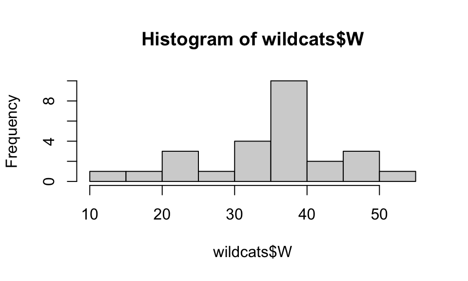
A basic histogram - of Linfield wins by season.

hist(wildcats$W)

When presenting data, we have a responsibility to make it readable, so we can do better than the above. We can supply titles, axis labels, annotations, colors, etc to help us visualize the data in a more useful way.

hist(wildcats$W,
     main="Wins by Season, Linfield Softball 1999-2020",
     xlab="Wins",
     col="purple",
     breaks=10
     )

We specify the bins in a histogram with the breaks option. If we have too few bins for the data, we lose all sorts of information, and if we have too many bins we might have a harder time seeing the shape of the distribution through the noise.

Boxplots

A boxplot is a visual representation of the 5 number summary, and R loves to make them!

Here’s a boxplot in its simplest form.

boxplot(wildcats$W)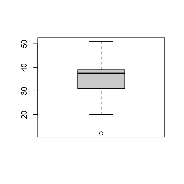

By default a boxplot is presented vertically, but we can ask for a horizontal boxplot as well, and we can add a splash of color.

boxplot(wildcats$W,
        main="Linfield softball wins by season (1999-2020)",
        col="red",
        horizontal = TRUE)

AND, we can add text to a graph. For instance, we can add the values in the 5 number summary to the boxplot, which gives more precision to the plot!

boxplot(wildcats$W,
        main="Linfield softball wins by season (1999-2020)",
        col="red",
        horizontal = TRUE)
v<-fivenum(wildcats$W)
text(x=c(v[1:5]),y=c(rep(1.3,5)),c(v[1:5]),cex=.7,col="purple")

Barplots

For categorical variables it can be useful to make barplots of counts. If we’re considering a vector of values we use the barplot() command in conjuntion with the table() command

barplot(table(wildcats$District),main="Finish at Districts",ylab="count",xlab="finish",col="#F5D7FB")

Choosing plot colors

If you type colors() at the console prompt you can get a list of names of built in colors.

You can find color codes on-line too, such as the one I used in the barplot code. Here’s one site for this: https://htmlcolorcodes.com/.

Scatter plots

A scatter plot is a useful way to visualize the relationship between two numeric variables. Here’s a scatter plot in its simplest form.

plot(x=wildcats$Year,y=wildcats$W)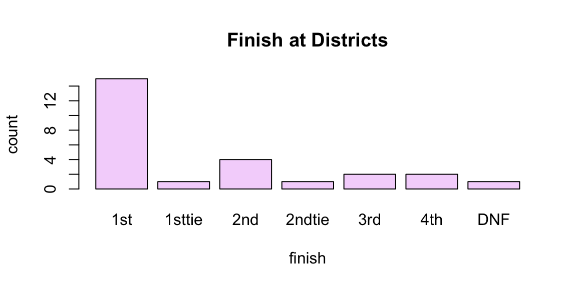

We can change the shape of points in a plot with the pch option, and change the scale of the y-axis.

plot(x=wildcats$Year,y=wildcats$W,
     main="Linfield softball wins by season", 
     ylab="wins",
     xlab="season",
     col="brown3",
     ylim=c(0,60),
     pch=16)

A quick guide to pch and point shapes (google “R pch options” for more details):

As an aside, we can create a line plot as well, by specifying type="l" (that’s an ‘l’ for ‘line’, not the number 1).

plot(x=wildcats$Year,y=wildcats$W,
     main="Linfield softball wins by season", 
     ylab="wins",
     xlab="season",
     col="purple",
     ylim=c(0,60),
     type="l")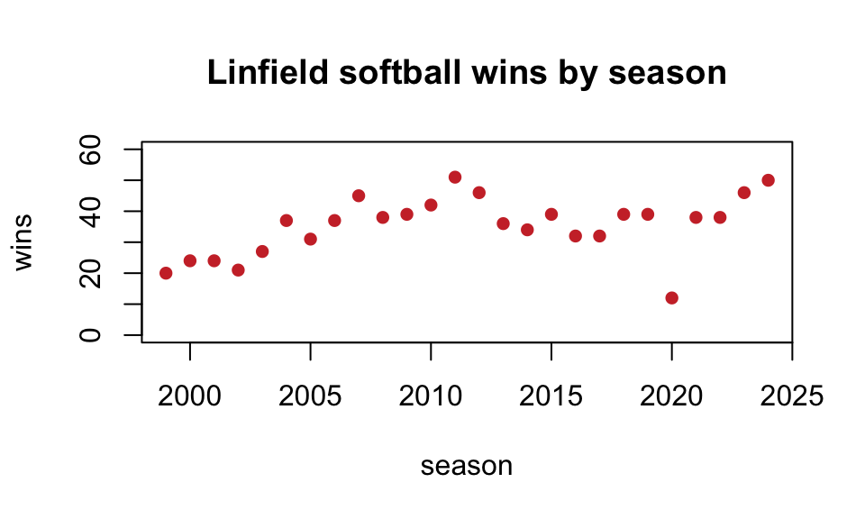

A little EDA (exploratory data analysis)

Let’s investigate the faithful data that comes in R.

dim(faithful) # This gives the number of rows (observations) and columns (variables)

## [1] 272   2

This data frame has 272 rows and 2 columns. What are the variables?

colnames(faithful)

## [1] "eruptions" "waiting"

The help tab (in the lower right pane) gives information about this data frame (type faithful in the search box.) The variable eruptions gives the duration of an eruption (in minutes), and the second variable, waiting, gives the waiting period (in minutes) until the next eruption.

We can ask for the first 7 rows of the data frame:

head(faithful,7)

##   eruptions waiting
## 1     3.600      79
## 2     1.800      54
## 3     3.333      74
## 4     2.283      62
## 5     4.533      85
## 6     2.883      55
## 7     4.700      88

We can extract the entry in row 6, column 2:

faithful[6,2]

## [1] 55

We can extract the subset of all the data for which the eruption value is at least 5 minutes:

subset(faithful, eruptions >= 5)

##     eruptions waiting
## 76      5.067      76
## 149     5.100      96
## 151     5.033      77
## 168     5.000      88

Only 4 of the 272 eruptions exceeded 5 minutes. Seems like a rare event!

A histogram of eruption duration:

hist(faithful$eruptions,
     main="Old Faithful Eruptions",
     xlab="Duration (minutes)",
     col="wheat"
     )

A scatter plot:

plot(x=faithful$eruptions, y=faithful$waiting,
     main="Old Faithful Eruptions",
     ylab="Wait time (minutes)",
     xlab="Duration (minutes)",
     pch=16,
     col="wheat"
     )

Test your understanding

Below are some bits of code. Can you see what information it will provide?

What does this code give?

max(wildcats$W)

## [1] 51

ANSWER: The maximum number of wins in a season over this time period.

Which season was this? Here’s a way to extract the entire season (row) from the data matrix that had the most number of wins:

subset(wildcats, W == max(wildcats$W))

##    Year           Coach  W L T District NCAA GP
## 13 2011 Jackson Vaughan 51 3 0      1st  1st 54

Wow! What a season! 51 wins against just 3 losses, first in districts, and National Champions!

What does this code give?

table(wildcats$NCAA)

## 
##     1st 2nd 3rd 4th 
##  18   2   2   1   1

ANSWER: It specifies how well Linfield did at Nationals over the 1999-2020 time period. Linfield has finished 1st twice, 2nd twice, 3rd once, and 4th once. The other 16 seasons they didn’t finish as high as 4th.

What does this code give?

sum(wildcats$District=="1st")

## [1] 13

ANSWER: It gives the number of seasons from 1999-2020 in which Linfield was 1st in the District

What does this code give?

wildcats$winpct <- wildcats$W/wildcats$GP

ANSWER: It creates a new column in the data frame wildcats called winpct. This column records the winning percentage for the team each season (wins divided by games played).

What does this code give?

max(wildcats$winpct)

## [1] 0.9444444

ANSWER: It returns the best winning percentage for a season between 1999 and 2020.

Which season was this?

subset(wildcats, winpct == max(wildcats$winpct))

##    Year           Coach  W L T District NCAA GP    winpct
## 13 2011 Jackson Vaughan 51 3 0      1st  1st 54 0.9444444

Not surprisingly, the best winning percentage occurred in the magical 2011 season in which the team went 51-3.

What does this code give?

plot(x=wildcats$L, y=wildcats$W,cex=.7,
     main="Linfield Softball (1999-2020)",
     xlab="Losses",
     ylab="Wins")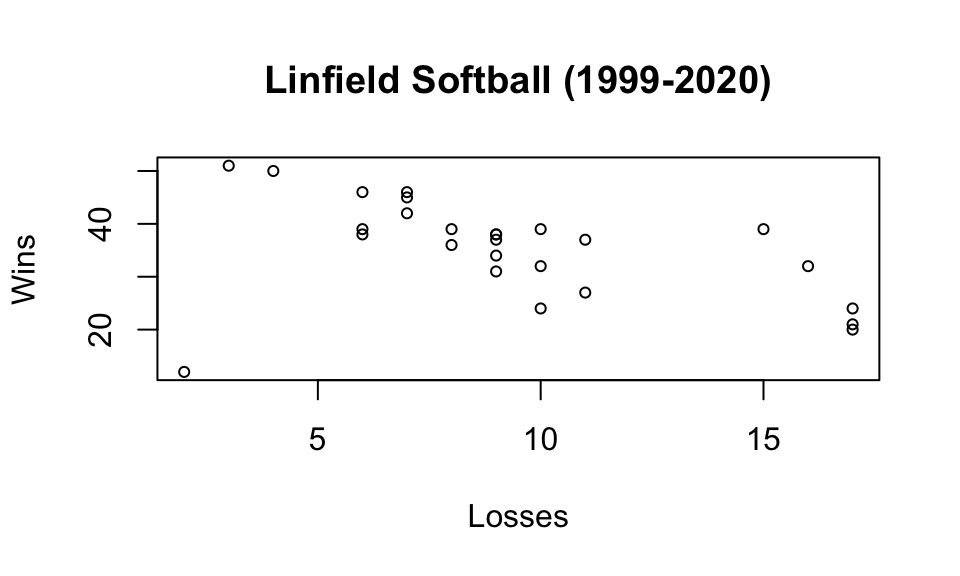

ANSWER: Scatterplot of wins vs losses. This plot makes it clear that 2020 was a strange season (the point in the lower left corner). This visual deviation from the trend indicates that something “different” was going on. What was it? (global pandemic!)

What does this code give?

fivenum(wildcats$W[wildcats$Coach=="Jackson Vaughan"])

## [1] 12 32 38 39 51

ANSWER: This code gives the 5 number summary for the Linfield softball wins for just the seasons in the data set in which the coach was Jackson Vaughan. More generally, consider this code, which makes use of the aggregate() method:

aggregate(wildcats$W, by=list(wildcats$Coach), FUN = median)

##           Group.1  x
## 1 Jackson Vaughan 38
## 2     Laura Kenow 24

The aggregate() method executes a function on a variable that has been grouped by a categorical variable. In the code above we have chosen to determine the median number of wins for each coach over this time period.

How about this one? x is a vector of three values, xbar is the mean of the values in x. What is v?

x = c(10,12,17)
xbar = mean(x)
v = sum((x - mean(x))^2)/(length(x)-1)
v

## [1] 13

ANSWER: This code reproduces the formula for the variance of a set of numbers:\[s^2 = \frac{1}{n-1}\sum_{i=1}^n(x_i-\overline{x})^2.\] Convinced? let’s check that this really gives the variance of the data set x:

var(x)

## [1] 13

Yup.

MATH 140: Using RStudio